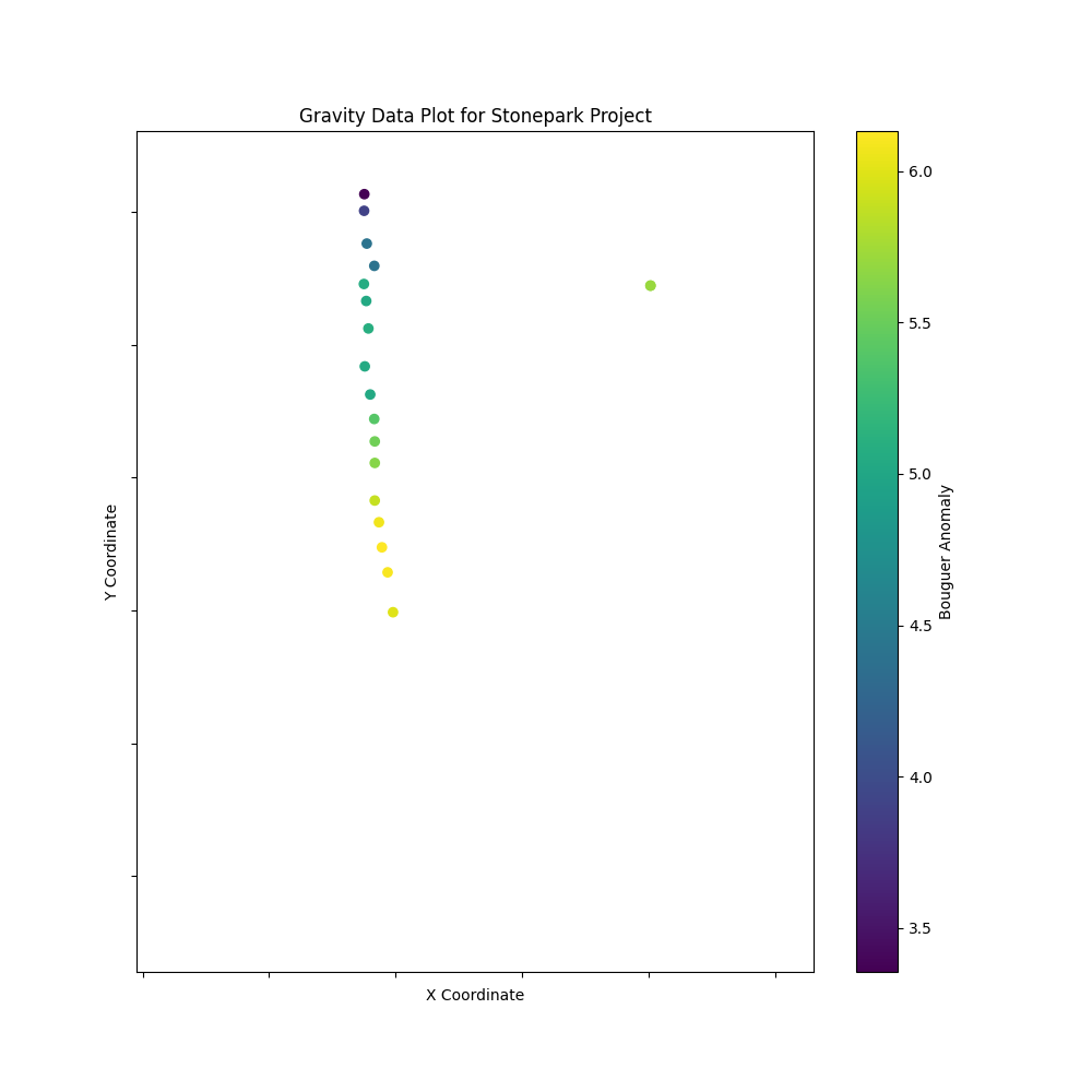
Gravity Data Visualization

This example illustrates how to read gravity data from the Stonepark project and visualize it. The data is converted for subsurface analysis.

import numpy as np
import pandas as pd
import matplotlib.pyplot as plt

# Import additional necessary libraries
from dotenv import dotenv_values

# Load environment variables and file path
config = dotenv_values()
path = config.get("PATH_TO_MODEL_1_BOUGUER")

# Read the data into a pandas DataFrame
df = pd.read_csv(path, sep=',', header=0)

# Selecting the columns of interest
interesting_columns = df[['X', 'Y', 'Bouguer_267_complete']]

# Define the extent of the observation area
omf_extent = np.array([559902.8297554839, 564955.6824703198 * 1.01, 644278.2600910577,
                       650608.7353560531, -1753.4, 160.3266042185512])

Plot the gravity data

plt.figure(figsize=(10, 10))
plt.scatter(df['X'], df['Y'], c=df['Bouguer_267_complete'], cmap='viridis')
plt.title('Gravity Data Plot for Stonepark Project')
plt.xlabel('X Coordinate')
plt.ylabel('Y Coordinate')
plt.colorbar(label='Bouguer Anomaly')

# Set the extent of the plot
plt.xlim(omf_extent[0], omf_extent[1])
plt.ylim(omf_extent[2], omf_extent[3])

# Optional: Hide axis labels for a cleaner look
plt.gca().axes.xaxis.set_ticklabels([])
plt.gca().axes.yaxis.set_ticklabels([])

# Display the plot
plt.show()