Note
Go to the end to download the full example code
Modeling and Propagation of Petrophysical Data for Mining Exploration (2/3)
Cleaning and Filling the Gaps
Barcelona 25/09/24 GEO3BCN Manuel David Soto, Juan Alcalde, Adrià Hernàndez-Pineda, Ramón Carbonel
Introduction
The dispersion and scarcity of petrophysical data are well-known challenges in the mining sector. These issues are primarily driven by economic factors, but also by geological factors such as sedimentary cover, weathering, erosion, or the depth of targets, geotechnical issues (e.g., slope or borehole stability), and even technical limitations or availability that have been resolved in other industries (for instance, sonic logs were not previously acquired due to a lack of interest in velocity field data).
To address the challenge of sparse and incomplete petrophysical data in the mining sector, we have developed three Jupyter notebooks that tackle these issues through a suite of open-source Python tools. These tools support researchers in the initial exploration, visualization, and integration of data from diverse sources, filling gaps caused by technical limitations and ultimately enabling the complete modeling of missing properties (through standard and more advanced ML-based models). We applied these tools to both recently acquired and legacy petrophysical data of two cores northwest of Collinstown (County Westmeath, Province of Leinster), Ireland, located 26 km west-northwest of the Navan mine. However, these tools are adaptable and applicable to mining data from any location.
After the EDA and integration of the petrophysical dataset of Collinstown (notebook 1/3), this second notebook gathers different tasks that can be grouped into what is called, in data science, data mining. These tasks are:
Record the positions of the original NaNs.
Record the positions and the values of the anomalies to be deleted.
Delete the anomalies.
Fill out all NaNs, both original and those resulting from deleting the anomalies, using different means (imputations, empirical formulas, simple ML models).
Compare the effectiveness of the different filling gap methods.
Use the better option to fill in the gaps and deliver the corrected petrophysical data for further investigation.
As with the previous notebook, these tasks are performed with open-source Python tools that are easily accessible by any researcher through a Python installation connected to the Internet.
Variables
The dataset used in this notebook is the ‘features’ dataset from the previous notebook (1/3). It contains the modelable petrophysical features with their respective anomalies. ‘Hole’ (text object) and ‘Len’ (float) variables are for reference, ‘Form’ (text object) is a categorical variable representing the major formations:
Name |
Explanation |
Unit |
|---|---|---|
Hole |
Hole name |
|
From |
Top of the sample |
m |
Len |
Length of the core sample |
cm |
Den |
Density |
g/cm³ |
Vp |
Compressional velocity |
m/s |
Vs |
Shear velocity |
m/s |
Mag |
Magnetic susceptibility |
|
Ip |
Chargeability or induced polarization |
mv/V |
Res |
Resistivity |
ohm·m |
Form |
Major formations or zone along the hole |
Libraries
The following are the Python libraries used along this notebook. PSL are Python Standard Libraries, UDL are User Defined Libraries, and PEL are Python External Libraries:
PLS
import sys
import warnings

# UDL
from vector_geology import basic_stat, geo

# PEL- Basic
import numpy as np
import pandas as pd
from tabulate import tabulate

# PEL - Plotting
import matplotlib.pyplot as plt
import seaborn as sns

# PEL - Data selection, transformation, preprocessing
from sklearn.model_selection import train_test_split
from sklearn.preprocessing import StandardScaler
from sklearn.preprocessing import PolynomialFeatures

# PEL - Imputer
from sklearn.impute import KNNImputer, SimpleImputer
from sklearn.experimental import enable_iterative_imputer
from sklearn.impute import IterativeImputer

# PEL- ML algorithms
from scipy.optimize import curve_fit
from sklearn.linear_model import LinearRegression, Lasso, Ridge
from sklearn.svm import SVR
from sklearn.neighbors import KNeighborsRegressor
from sklearn.tree import DecisionTreeRegressor
from sklearn.ensemble import RandomForestRegressor, GradientBoostingRegressor
from sklearn import tree
import xgboost as xgb

# PEL - Metrics
from sklearn.metrics import mean_squared_error, mean_absolute_error, r2_score
Settings
Seed of random process
seed = 123

# Warning suppression
warnings.filterwarnings("ignore")
Data Loading
Features data load
features = pd.read_csv('Output/features.csv', index_col=0)
features.head()
features.describe()
Columns in the features dataframe
features.columns
Index(['Hole', 'From', 'Len', 'Den', 'Vp', 'Vs', 'Mag', 'Ip', 'Res', 'Form'], dtype='object')
Features Cleaning
The plots below show the anomalous values of the four affected variables. Then, along the section, we will register the position of the anomalies and then delete them, according to the findings of the previous notebook (1/3):
Feat. |
Deliting Anomalies |
|---|---|
Den |
Values above 4 g/cm³ are related to bad measurements in core samples longer than 11.2 cm. |
Vp |
Values below 3000 m/s are related to fractures in the core samples. |
Vs |
Values less than 1000 m/s are also related to core fractures. |
Mag |
The anomaly of 93.9 is above the range of the measuring equipment. |
Ip |
We see no reasons to discard outliers. |
Res |
We see no reasons to discard outliers. |
Bad data areas in Vp, Vs, Mag vs. Den
plt.figure(figsize=(16, 5))

# len vs. Den
plt.subplot(131)
plt.scatter(features.Vp, features.Den, alpha=0.65, edgecolors='k', c='skyblue')
plt.axhspan(4, 5.25, color='r', alpha=0.2)
plt.axvspan(500, 3000, color='r', alpha=0.2)
plt.text(1100, 4.7, 'Bad Data Area')
plt.axis([500, 7000, 2, 5.25])
plt.xlabel('Vp (m/s)')
plt.ylabel('Den (g/cm3)')
plt.grid()

# Den vs. Vs bad data area
plt.subplot(132)
plt.scatter(features.Vs, features.Den, alpha=0.65, edgecolors='k', c='skyblue')
plt.axhspan(4, 5.25, color='r', alpha=0.2)
plt.axvspan(0, 1000, color='r', alpha=0.2)
plt.text(75, 4.7, 'Bad Data Area')
plt.axis([0, 4000, 2, 5.25])
plt.xlabel('Vs (m/s)')
plt.ylabel('Den (g/cm3)')
plt.grid()

# Den vs. Vs bad data area
plt.subplot(133)
plt.scatter(features.Mag, features.Den, alpha=0.65, edgecolors='k', c='skyblue')
plt.axvspan(20, 100, color='r', alpha=0.2)
plt.axhspan(4, 5.25, color='r', alpha=0.2)
plt.text(2, 4.7, 'Bad Data Area')
plt.axis([-5, 100, 2, 5.25])
plt.xlabel('Magnetic Susceptibility')
plt.ylabel('Den (g/cm3)')
plt.grid()

plt.suptitle('Variable with Anomalies in the Keywells')

plt.tight_layout();

NaN and Anomalies Preservation
The folowing dataframes preserves the location of original NaN (1) and anomalies (2):
nan_ano_loc = features.copy()
Fill the datafreme with 1 and 2
for column in features.columns:
    nan_ano_loc[column] = np.where(pd.isna(features[column]), 1, 0)

nan_ano_loc.Den = np.where(features.Den > 4, 2, 0)
nan_ano_loc.Vp = np.where(features.Vp < 3000, 2, 0)
nan_ano_loc.Vs = np.where(features.Vs < 1000, 2, 0)
nan_ano_loc.Mag = np.where(features.Mag > 20, 2, 0)
nan_ano_loc.head()
nan_ano_loc.describe()
Save the locations of nans and anomalies
nan_ano_loc.to_csv('Output/nan_ano_loc.csv')
Preservation of the anomalies
anomalies = features[features.Den > 4]
anomalies = pd.concat([anomalies, features[features.Vp < 3000]])
anomalies = pd.concat([anomalies, features[features.Vs < 1000]])
anomalies = pd.concat([anomalies, features[features.Mag > 2]])
anomalies = anomalies.drop_duplicates().sort_index()
anomalies
Number and % of anomalies by boreholes
print('Total anomalies:', len(anomalies), '({:.1f}%)'.format(100 * len(anomalies) / (features.shape[0] * features.shape[1])))
anomalies.Hole.value_counts()
Total anomalies: 18 (0.5%)

Hole
TC-1319-005    12
TC-3660-008     6
Name: count, dtype: int64
Save the anomalies
anomalies.to_csv('Output/anomalies.csv')
Rows with anomalies
list(anomalies.index)
[0, 1, 3, 6, 7, 11, 12, 13, 24, 77, 79, 159, 174, 198, 243, 248, 305, 312]
Anomalies Deletion
features2, new features dataframe without anomalies
features2 = features.copy()

features2['Den'] = np.where(features.Den > 4, np.nan, features.Den)
features2['Vp'] = np.where(features.Vp < 3000, np.nan, features.Vp)
features2['Vs'] = np.where(features.Vs < 1000, np.nan, features.Vs)
features2['Mag'] = np.where(features.Mag > 20, np.nan, features.Mag)

features2.head()
features2.describe()
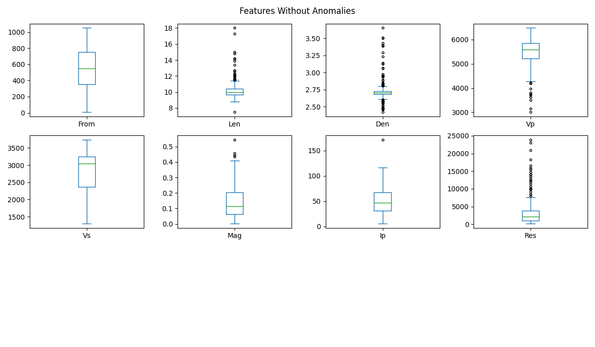
Boxplot of each feature without anomalies
features2.plot.box(subplots=True, grid=False, figsize=(12, 7), layout=(3, 4), flierprops={"marker": "."})
plt.suptitle('Features Without Anomalies')
plt.tight_layout();
Save features without anomalies
features2.to_csv('Output/features2.csv')
NaNs in the Features
Original NaNs
features.isna().sum()
Hole     0
From     0
Len      8
Den      2
Vp      19
Vs      40
Mag      3
Ip      26
Res     26
Form     0
dtype: int64
Total original NaNs
features.isna().sum().sum()
np.int64(124)
% of original NaNs
features.isna().sum() / len(features) * 100
Hole     0.000000
From     0.000000
Len      2.431611
Den      0.607903
Vp       5.775076
Vs      12.158055
Mag      0.911854
Ip       7.902736
Res      7.902736
Form     0.000000
dtype: float64
Total % original and new NaNs
print('% NaN in Features:', round(100 * features.isna().sum().sum() / (features.shape[0] * features.shape[1]), 1))
% NaN in Features: 3.8
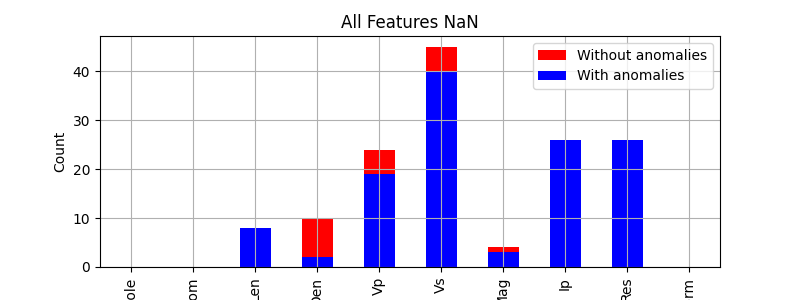
Original and new NaNs
features2.isna().sum()
Hole     0
From     0
Len      8
Den     10
Vp      24
Vs      45
Mag      4
Ip      26
Res     26
Form     0
dtype: int64
Total original and new NaNs
features2.isna().sum().sum()
np.int64(143)
Total % original and new NaNs
print('% NaN in features2:', round(100 * features2.isna().sum().sum() / (features2.shape[0] * features2.shape[1]), 1))
% NaN in features2: 4.3
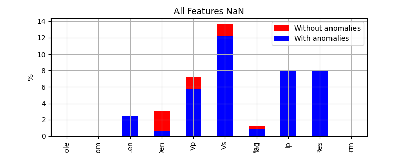
% Total original and new NaNs by feature
features2.isna().sum() / len(features) * 100
Hole     0.000000
From     0.000000
Len      2.431611
Den      3.039514
Vp       7.294833
Vs      13.677812
Mag      1.215805
Ip       7.902736
Res      7.902736
Form     0.000000
dtype: float64
Bar plot of NaNs
features2.isna().sum().plot.bar(figsize=(8, 3), color='r', ylabel='Count', title='All Features NaN', label='Without anomalies', legend=True)
features.isna().sum().plot.bar(figsize=(8, 3), color='b', label='With anomalies', legend=True, grid=True)
<Axes: title={'center': 'All Features NaN'}, ylabel='Count'>
Bar plot of NaNs (%)
(features2.isna().sum() / len(features) * 100).plot.bar(figsize=(8, 3), color='r', label='Without anomalies', legend=True)
(features.isna().sum() / len(features) * 100).plot.bar(figsize=(8, 3), color='b', label='With anomalies', legend=True,
                                                       title='All Features NaN', ylabel='%', grid=True);
<Axes: title={'center': 'All Features NaN'}, ylabel='%'>
Total rows at least one with NaN and their indexes
total_nan_index = list(features2[pd.isna(features2).any(axis=1)].index)
print('Total rows with at least one NaN:', len(total_nan_index), '\n', '\n', 'Rows indexes:')
total_nan_index
Total rows with at least one NaN: 62

 Rows indexes:

[0, 1, 3, 6, 7, 11, 12, 13, 15, 24, 36, 45, 47, 63, 68, 71, 75, 77, 79, 99, 100, 105, 110, 111, 112, 113, 114, 115, 117, 118, 135, 158, 159, 160, 164, 174, 183, 185, 187, 189, 191, 194, 197, 198, 201, 206, 209, 210, 229, 233, 240, 243, 248, 251, 276, 305, 311, 312, 318, 319, 320, 325]
Filling the holes
Imputations Evaluation
Imputation refers to the alternative process of filling in all the missing values (NaN) or gaps in a dataset. Instead of removing rows or columns with missing values, those values are replaced (imputed) with estimated values based on information available in the entire dataset (in all variables). This is typically done when you want to preserve the other values in the rows where the NaNs are, and when the missing values for each variable or column do not exceed 25%.
Since multiple imputation methods are available, it’s important to evaluate each one and select the method that yields the best results, based on metrics such as the sum of residuals, MAE, MSE, RMSE, and R² (formulas of these metrics in the annex). In this case, we tested six imputation methods:
Simple mean (mean)
Simple K-Means (knn)
Iterative Impute (ii)
Normalized mean (nmean)
Normalized K-Means (nknn)
Normalized Iterative Imputer (nii)
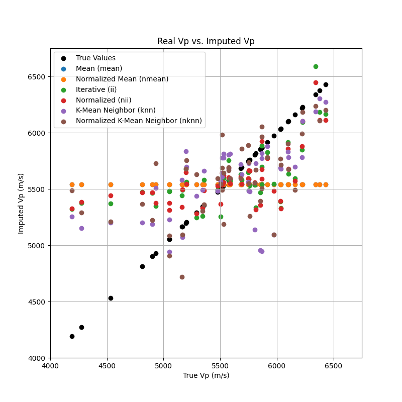
To compare these methods, we first created fictitious gaps in the Vp values (just this variable due to its importance, and for simplicity and speed) of a non-NaN dataset to compare them later the real values of Vp against the imputed. By doing so, we can compute each method’s metrics and determine which performs best. In addition to these metrics, at the end of the section, there is a plot with the resulting values of each imputer method with respect to the real values, showing less dispersion towards the top of the plot.
Non-NaN dataframe to test the imputation
features2_num = features2[['From', 'Den', 'Vp', 'Vs', 'Mag', 'Ip', 'Res']]
features2_num_nonan = features2_num.dropna()
features2_num_nonan.head()
Generation of random mask for the fictitious NaNs or gaps
np.random.seed(seed)
missing_rate = 0.2  # Porcentaje de valores faltantes
Vp_mask = np.random.rand(features2_num_nonan.shape[0]) < missing_rate
Vp_mask
array([False, False, False, False, False, False, False, False, False,
       False, False, False, False,  True, False, False,  True,  True,
       False, False, False, False, False, False, False, False, False,
       False, False, False,  True, False, False, False, False, False,
       False, False, False, False, False,  True, False, False, False,
       False, False, False, False, False,  True, False, False, False,
       False, False, False, False, False, False, False, False, False,
       False, False,  True, False, False,  True, False,  True, False,
       False, False,  True, False, False,  True,  True, False, False,
       False, False, False, False, False, False,  True, False, False,
       False, False, False, False, False, False,  True, False, False,
       False, False, False,  True,  True, False, False, False, False,
       False, False, False, False,  True, False, False, False, False,
       False,  True, False, False, False, False, False, False, False,
       False, False, False, False, False,  True, False, False, False,
        True, False, False, False, False,  True, False, False, False,
       False, False, False,  True, False, False,  True, False, False,
       False, False,  True, False, False, False, False, False, False,
       False,  True, False, False, False, False, False, False, False,
        True, False, False, False,  True,  True,  True, False, False,
       False,  True, False, False, False, False,  True, False, False,
       False, False, False, False, False,  True, False,  True, False,
       False,  True, False,  True, False, False, False, False,  True,
       False, False,  True, False, False, False, False, False, False,
        True, False, False,  True, False, False, False, False, False,
        True, False, False, False,  True, False,  True, False, False,
       False,  True, False, False, False, False,  True, False, False,
       False,  True, False, False, False, False, False, False, False,
       False, False,  True, False, False, False,  True, False, False,
        True, False, False, False, False,  True])
New gaps in Vp of the Non-NaN dataframe
features2_new_missing = features2_num_nonan.copy()
features2_new_missing.loc[Vp_mask, 'Vp'] = np.nan
features2_new_missing
At index 328 the original Vp is
features.loc[328]
Hole    TC-3660-008
From          833.4
Len            10.1
Den           2.735
Vp           5805.0
Vs           3217.0
Mag           0.308
Ip            33.86
Res          2300.0
Form            PAL
Name: 328, dtype: object
True Vp values
true_vp = features2_num_nonan[Vp_mask].Vp.reset_index(drop=True)
true_vp.head()
0    5196.0
1    6159.0
2    6037.0
3    5815.0
4    4930.0
Name: Vp, dtype: float64
Evaluation of the imputers
# List of imputers
imputers = []

# Initialize imputers
mean_imputer = SimpleImputer(strategy='mean')
ii_imputer = IterativeImputer(max_iter=10, random_state=seed)
knn_imputer = KNNImputer(n_neighbors=5)

# Normalization
scaler = StandardScaler()
features2_new_missing_scaled = scaler.fit_transform(features2_new_missing)

# Append of imputer (name, norm, imputer, data)
imputers.append(('mean', 'no', mean_imputer, features2_new_missing))
imputers.append(('ii', 'no', ii_imputer, features2_new_missing))
imputers.append(('knn', 'no', knn_imputer, features2_new_missing))
imputers.append(('nmean', 'yes', mean_imputer, features2_new_missing_scaled))
imputers.append(('nii', 'yes', ii_imputer, features2_new_missing_scaled))
imputers.append(('nknn', 'yes', knn_imputer, features2_new_missing_scaled))

# Results table
headers = ['Imputer', 'Normalization', 'Sum Residual', 'MAE', 'MSE', 'RMSE', 'R2']
rows = []

# Loop over the imputers
for name, norm, imputer, data in imputers:
    # Impute the data
    imputed_data = imputer.fit_transform(data)

    # Reverse the normalization if data was normalized
    if norm == 'yes':
        imputed_data = scaler.inverse_transform(imputed_data)

    # Convert the array to dataframe
    imputed_data_df = pd.DataFrame(imputed_data, columns=features2_new_missing.columns)
    imputed_vp = imputed_data_df.loc[Vp_mask, 'Vp'].reset_index(drop=True)

    # Calculate residuals and metrics
    residual = sum(true_vp - imputed_vp)
    mae = mean_absolute_error(true_vp, imputed_vp)
    mse = mean_squared_error(true_vp, imputed_vp)
    rmse = np.sqrt(mse)
    r2 = r2_score(true_vp, imputed_vp)

    # Create a dataframe for imputer using globals()
    globals()[f'imputer_{name}'] = imputed_data_df.copy()

    # Append results
    rows.append([name, norm, residual, mae, mse, rmse, r2])

# Print the results in a formatted table

print('Seed:', seed)

print(tabulate(rows, headers=headers, tablefmt="fancy_outline"))
Seed: 123
╒═══════════╤═════════════════╤════════════════╤═════════╤════════╤═════════╤═════════════╕
│ Imputer   │ Normalization   │   Sum Residual │     MAE │    MSE │    RMSE │          R2 │
╞═══════════╪═════════════════╪════════════════╪═════════╪════════╪═════════╪═════════════╡
│ mean      │ no              │        1779.8  │ 394.903 │ 256363 │ 506.323 │ -0.00517294 │
│ ii        │ no              │       -1106.23 │ 308.72  │ 163029 │ 403.768 │  0.360781   │
│ knn       │ no              │        -490.6  │ 310.118 │ 168360 │ 410.317 │  0.339878   │
│ nmean     │ yes             │        1779.8  │ 394.903 │ 256363 │ 506.323 │ -0.00517294 │
│ nii       │ yes             │        -646.02 │ 296.29  │ 160690 │ 400.862 │  0.36995    │
│ nknn      │ yes             │        -924.4  │ 298.808 │ 166131 │ 407.592 │  0.348616   │
╘═══════════╧═════════════════╧════════════════╧═════════╧════════╧═════════╧═════════════╛
imputer_nii.head()
Plot of the real Vp vs. the imputed Vp
plt.figure(figsize=(8, 8))
plt.scatter(true_vp, true_vp, color='k', label='True Values')
plt.scatter(true_vp, imputer_mean[Vp_mask].Vp, label='Mean (mean)')
plt.scatter(true_vp, imputer_nmean[Vp_mask].Vp, label='Normalized Mean (nmean)')
plt.scatter(true_vp, imputer_ii[Vp_mask].Vp, label='Iterative (ii)')
plt.scatter(true_vp, imputer_nii[Vp_mask].Vp, label='Normalized (nii)')
plt.scatter(true_vp, imputer_knn[Vp_mask].Vp, label='K-Mean Neighbor (knn)')
plt.scatter(true_vp, imputer_nknn[Vp_mask].Vp, label='Normalized K-Mean Neighbor (nknn)')
plt.xlabel('True Vp (m/s)')
plt.ylabel('Imputed Vp (m/s)')
plt.title('Real Vp vs. Imputed Vp')
plt.axis([4000, 6750, 4000, 6750])
plt.legend()
plt.grid()
plt.show()
- Best Imputation
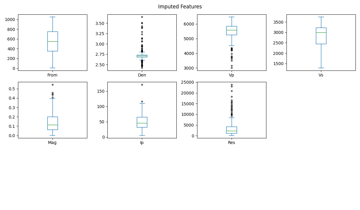
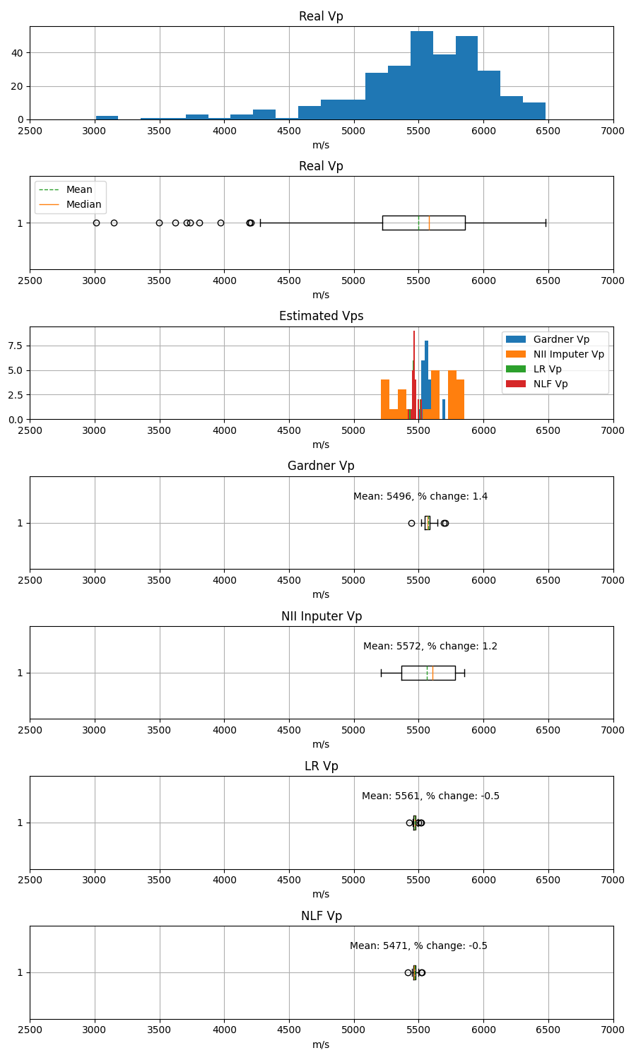
By a closer examination of the metrics, we can conclude that the normalized Iterative Imputer (nii), also called MICE (Multiple Imputation by Chained Equations), performs the best (or least poorly), particularly for the Vp variable, with the mean of the imputed values increasing just 1.2 % with respect to the mean of the real values. Consequently, we used the nii imputer to fill the gaps across all variables and saved the updated dataset in a new dataframe (features3).
The multiplot of this section shows that the imputation process maintains the shape of the boxplot of the variables from which the anomalies have been removed. In other words, this multiplot of the imputed dataset (features3) is almost identical to the multiplot of features2 in section 7.2.
Normalized interactive imputation of features2
# Data normalization
scaler = StandardScaler()
features2_scaled = scaler.fit_transform(features2_num)

# Imputation of normalized data
nii_features3_array = ii_imputer.fit_transform(features2_scaled)

# Reverse normalization and new imputed dataframe
features3 = pd.DataFrame(scaler.inverse_transform(nii_features3_array), columns=features2_num.columns)

features3.head()
features3.describe()
Boxplot of each imputed feature
features3.plot.box(subplots=True, grid=False, figsize=(12, 7), layout=(3, 4), flierprops={"marker": "."})
plt.suptitle('Imputed Features')
plt.tight_layout()
Copy reference variable to features3
features3[['Hole', 'Len', 'Form']] = features2[['Hole', 'Len', 'Form']]
Order of the variables
features3_series = list(features2.columns)
features3_series
['Hole', 'From', 'Len', 'Den', 'Vp', 'Vs', 'Mag', 'Ip', 'Res', 'Form']
Reordering features3
features3 = features3[features3_series]
features3.head()
Save features3
features3.to_csv('Output/features3.csv')
Indixes of Vp values in features2
features2.Vp[~features2.Vp.isna()]
1      5514.0
2      5754.0
3      5773.0
4      6034.0
5      4661.0
        ...
323    5621.0
324    5680.0
326    5593.0
327    5858.0
328    5805.0
Name: Vp, Length: 305, dtype: float64
Indixes of Vp NaNs in features2
features2.Vp[features2.Vp.isna()]
0     NaN
15    NaN
36    NaN
77    NaN
79    NaN
111   NaN
118   NaN
159   NaN
174   NaN
183   NaN
185   NaN
187   NaN
189   NaN
191   NaN
194   NaN
201   NaN
210   NaN
233   NaN
240   NaN
251   NaN
276   NaN
311   NaN
320   NaN
325   NaN
Name: Vp, dtype: float64
Vp_nan_index = list(features2.Vp[features2.Vp.isna()].index)
Vp_nan_index
[0, 15, 36, 77, 79, 111, 118, 159, 174, 183, 185, 187, 189, 191, 194, 201, 210, 233, 240, 251, 276, 311, 320, 325]
Original Vp without anomalies
features2.Vp.describe()
count     305.000000
mean     5496.386885
std       556.077848
min      3009.000000
25%      5220.000000
50%      5581.000000
75%      5858.000000
max      6478.000000
Name: Vp, dtype: float64
Imputed Vp
features3.Vp.iloc[Vp_nan_index].describe()
count      24.000000
mean     5560.948607
std       225.846356
min      5210.315493
25%      5369.531486
50%      5605.088801
75%      5779.916352
max      5854.418200
Name: Vp, dtype: float64
% of increase of the mean of the imputed Vp compared with the real Vp
vp_change_den = 100 * (features3.Vp.iloc[Vp_nan_index].mean() - features2.Vp.mean()) / features2.Vp.mean()
print('Increase of the mean:', '{:.1f} %'.format(vp_change_den))
Increase of the mean: 1.2 %
nii Vp for comparison
nii_vp = features3.Vp.iloc[Vp_nan_index]
nii_vp.head()
0     5725.879959
15    5604.870331
36    5558.402401
77    5374.912754
79    5210.315493
Name: Vp, dtype: float64
Estimating Vp
The calculation of a single variable such as Vp (again, just this variable due to its importance, for simplicity and speed) allows us to try and evaluate different methods for filling the gaps, from empirical formulas to the simplest Machine Learning (ML) algorithms.
Vp by Gardner
The Gardner’s formula is a well-known empirical formula that allows us to transform the density (Den) into compressional velocity (Vp):
Where
\(\phi\) is the density and the standard coefficients (reference: https://wiki.seg.org/wiki/Dictionary:Gardner%E2%80%99s_equation) are:
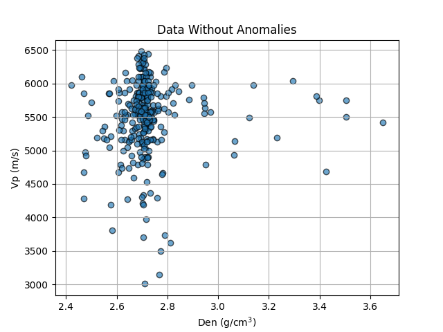
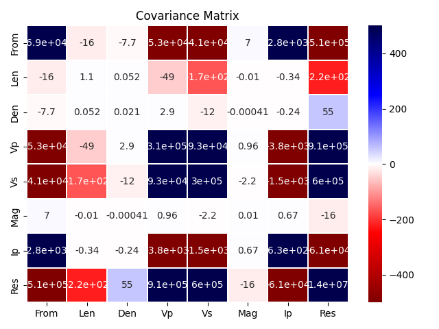
Contrary to the expected increasing trend between Den and Vp, the plot below shows an anomalous vertical trend, where multiple Vp values are associated with a single Den value (around 2.7). This anomalous trend results in a negative R² (-0.021, the worst so far) when Vp is calculated using all values, and this score improves slightly when we filter out the pairs that fall outside the expected increasing trend. This is confirmed by the low covariance presented by the Den-Vp pair in the covariance matrix of this section (low correlation coefficient in the previous notebook 1/3). %% Plot of Den vs. Vp
plt.grid()
plt.scatter(features2.Den, features2.Vp, alpha=0.65, edgecolors='k')
plt.xlabel('Den (g/cm$^3$)')
plt.ylabel('Vp (m/s)')
plt.title('Data Without Anomalies')
Text(0.5, 1.0, 'Data Without Anomalies')
features2.select_dtypes(include=['number'])
Covariance of the features2
vari_mat = features2.select_dtypes(include=['number']).cov()
vari_mat
vari_mat.describe()
Covariance matrix
sns.heatmap(vari_mat, vmin=-500, vmax=500, center=0, linewidths=.1, cmap='seismic_r', annot=True)
plt.title('Covariance Matrix')
plt.tight_layout()
plt.show()
Gardner Vp in features2, with the standard alpha of 4348
features2['VpG'] = 4348 * (features2.Den) ** 0.25
features2['VpG']
0      5526.493483
1              NaN
2      5903.741408
3              NaN
4      5857.165129
          ...
324    5605.763308
325    5547.023745
326    5605.256023
327    5626.444480
328    5591.506938
Name: VpG, Length: 329, dtype: float64
Drop NaNs for metrics calculation
features2_nonan = features2.dropna()
features2_nonan.head()
Metrics of the Gardner calculation with all values
vpg_metrics = basic_stat.metrics(features2_nonan.Vp, features2_nonan.VpG)

print("Metrics for Gardner:\n")
print(vpg_metrics)
Metrics for Gardner:

{'Sum of Residuals': np.float64(-10723.609649536735), 'MAE': np.float64(365.5125465596317), 'MSE': np.float64(254469.14816210992), 'RMSE': np.float64(504.44935143392735), 'R2': -0.021743605762918117}
Metrics of the Gardner calculation with filtered values
vpg_metrics2 = basic_stat.metrics(
    features2_nonan.Vp[(features2_nonan.Vp > 4000) & (features2_nonan.Vp < 6000)],
    features2_nonan.VpG[(features2_nonan.Vp > 4000) & (features2_nonan.Vp < 6000)]
)

print("Metrics for Gardner with Filtered Data Vp):\n")
print(vpg_metrics2)
Metrics for Gardner with Filtered Data Vp):

{'Sum of Residuals': np.float64(-25589.572721078162), 'MAE': np.float64(295.9254751013969), 'MSE': np.float64(162331.10374522334), 'RMSE': np.float64(402.9033429313082), 'R2': -0.0937786027043972}
Gardner Vp for comparison
gard_vp = features2.VpG.iloc[Vp_nan_index]
gard_vp.head()
0     5526.493483
15    5520.661324
36    5633.454391
77    5586.388848
79    5691.523695
Name: VpG, dtype: float64
Simpliest ML models for Vp
Machine Learning (ML) algorithms offer a wide range of options to calculate missing values of a single variable. From the simplest and most well-known, such as linear regression with an independent variable, to the most complex. Below we use the simplest ML algorithms and their respective metrics, applied again to predict Vp and fill its gaps. But first, we split the non-NaN portion of the filtered data (features2) for training and testing.
features2_num_nonan.head()
Target from filtered features2
# The target or objective of the model is the Vp
target = features2_num_nonan.Vp[(features2_num_nonan.Vp > 4000) & (features2_num_nonan.Vp < 6000)]
print(target.shape)
target.head()
(225,)

2     5754.0
5     4661.0
8     5815.0
9     4785.0
10    5707.0
Name: Vp, dtype: float64
Filtered density is the independent feature to compute Vp, the target
features2_den = features2_num_nonan.Den[(features2_num_nonan.Vp > 4000) & (features2_num_nonan.Vp < 6000)]
features2_den.head()
2     3.399
5     2.782
8     3.386
9     2.616
10    2.821
Name: Den, dtype: float64
Split and shape of data for training and testing
X_train, X_test, y_train, y_test = train_test_split(features2_den, target, test_size=0.2, random_state=seed)

X_train = np.array(X_train).reshape(-1, 1)
X_test = np.array(X_test).reshape(-1, 1)
y_train = np.array(y_train).reshape(-1, 1)
y_test = np.array(y_test).reshape(-1, 1)

print('X_train shape:', X_train.shape)
print('y_train shape:', y_train.shape)

print('X_test shape:', X_test.shape)
print('y_test shape:', y_test.shape)
X_train shape: (180, 1)
y_train shape: (180, 1)
X_test shape: (45, 1)
y_test shape: (45, 1)
Simple Linear Regression
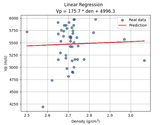
The linear regression is perhaps one of the simplest ML algorithms, it allows us to define a simple formula to compute Vp from Den, the only feature. The regression using all the data gave a negative $R^2$ (the predictions are worse than if it had simply predicted the mean), while applying a filter in the input data(4000 < Vp < 6000) resulted in a positive $R^2$, although a very small one (0.003).
Linear Regression
# Model training and prediction
lr_model = LinearRegression().fit(X_train, y_train)
lr_predict = lr_model.predict(np.array(X_test))

# Coheficients
coef = lr_model.coef_.item()
inter = lr_model.intercept_.item()
Metric of the linear regression with filtered data
lr_metrics = basic_stat.metrics(y_test, lr_predict)

print("Metrics for Linear Regressor:\n")
print(lr_metrics)
Metrics for Linear Regressor:

{'Sum of Residuals': np.float64(-663.6657176180624), 'MAE': np.float64(321.4070681962207), 'MSE': np.float64(152576.8824032091), 'RMSE': np.float64(390.61090922196365), 'R2': 0.002886141920427243}
Plot of filtered data and regression
plt.scatter(X_test, y_test, label='Real data', alpha=0.65, edgecolors='k')
plt.plot(X_test, lr_predict, c='r', label='Prediction')
plt.title(f"Vp = {coef:.1f} * den + {inter:.1f}")
plt.suptitle('Linear Regression')
plt.xlabel('Density (g/cm$^3$)')
plt.ylabel('Vp (m/s)')
plt.grid()
plt.legend();
<matplotlib.legend.Legend object at 0x7f3199fc2ce0>
lr Vp for comparison
#  Density of the Vp calculations
den_feature = np.array(features2.Den.iloc[Vp_nan_index]).reshape(-1, 1)

lr_vp = lr_model.predict(den_feature)
lr_vp
array([[5454.81134299],
       [5452.87886354],
       [5491.35277254],
       [5475.01453721],
       [5512.08300661],
       [5473.43341766],
       [5454.98702294],
       [5427.58095077],
       [5466.58189962],
       [5467.28461942],
       [5474.66317731],
       [5468.33869912],
       [5458.85198183],
       [5466.05485977],
       [5454.81134299],
       [5517.70476501],
       [5469.74413872],
       [5470.27117857],
       [5467.98733922],
       [5478.52813621],
       [5470.27117857],
       [5462.01422093],
       [5495.74477128],
       [5461.66286103]])
Non Linear Fit
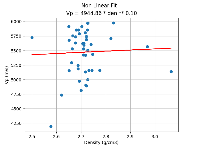
Although the non_linear fit is more powerful since it can fit the alpha and beta coefficients of a non-linear curve of density to Vp, the $R^2$ metric (0.004) does not differ much from the linear regression with the filtered data.
Reshaping the filtered data
X_train = np.array(X_train).flatten()
y_train = np.array(y_train).flatten()

print('X_train shape:', X_train.shape)
print('y_train shape:', y_train.shape)
X_train shape: (180,)
y_train shape: (180,)
Gardner function for double fitting, for alpha and beta
def gardner_model(X_train, alpha, beta):
    return alpha * X_train ** beta
Model fit
popt, pcov = curve_fit(gardner_model, X_train, y_train, p0=[0, 0]) # p0 is the initial estimation of alpha y beta
Coheficients and prediction
alpha, beta = popt

print('Alpha:', alpha)
print('Beta:', beta)

nlf_predict = gardner_model(X_test, alpha, beta)
Alpha: 4944.85723377095
Beta: 0.1017276747649569
Metric of the non linear fit with filtered data
nlf_metrics = basic_stat.metrics(y_test, nlf_predict)

print("Metrics for Non Linear Fit:\n")
print(nlf_metrics)
Metrics for Non Linear Fit:

{'Sum of Residuals': np.float64(-672.1847517458073), 'MAE': np.float64(321.430456631444), 'MSE': np.float64(152446.9582936085), 'RMSE': np.float64(390.4445649431024), 'R2': 0.003735216355170601}
Plot of filtered data and NLF equation
plt.scatter(X_test, y_test, label='Real data')
plt.plot(X_test, nlf_predict, c='r', label='Prediction')
plt.title(f"Vp = {alpha:.2f} * den ** {beta:.2f}")
plt.xlabel("Density (g/cm3)")
plt.suptitle('Non Linear Fit')
plt.ylabel("Vp (m/s)")
plt.grid()
plt.show()
nlf Vp for comparison
nlf_vp = gardner_model(den_feature, alpha, beta)
nlf_vp
array([[5451.77127868],
       [5449.42946455],
       [5494.46242706],
       [5475.7369865 ],
       [5517.43839526],
       [5473.89450644],
       [5451.98373102],
       [5417.92250818],
       [5465.84650885],
       [5466.67677416],
       [5475.32801939],
       [5467.92008814],
       [5456.63928719],
       [5465.22307824],
       [5451.77127868],
       [5523.52610545],
       [5469.57396647],
       [5470.19303406],
       [5467.50592748],
       [5479.81189483],
       [5470.19303406],
       [5460.42246055],
       [5499.40142812],
       [5460.00324939]])
Vps Comparison
The real Vp values allow us to evaluate the quality of different procedures that estimate Vp, such as different imputation algorithms, the Gardner empirical formula, and the simpliest ML regression model.
Datos y títulos a utilizar en el bucle
plt.figure(figsize=(9, 15))

# Histograms
plt.subplot(7, 1, 1)
plt.grid(zorder=2)
plt.hist(features2.Vp, bins=20, zorder=3)
plt.xlim(2500, 7000)
plt.xlabel('m/s')
plt.title('Real Vp')

plt.subplot(7, 1, 2)
box = plt.boxplot(features2.Vp.dropna(), vert=False, showmeans=True, meanline=True, patch_artist=False)
mean_line = box['means'][0]  # Obtener la línea de la media
median_line = box['medians'][0]  # Obtener la línea de la mediana
plt.legend([mean_line, median_line], ['Mean', 'Median'], loc='upper left')
plt.xlim(2500, 7000)
plt.title('Real Vp')
plt.xlabel('m/s')
plt.grid()

plt.subplot(7, 1, 3)
plt.grid(zorder=2)
plt.hist(gard_vp, label='Gardner Vp', zorder=4)
plt.hist(nii_vp, label='NII Imputer Vp', zorder=7)
plt.hist(lr_vp, label='LR Vp', zorder=9)
plt.hist(nlf_vp, label='NLF Vp', zorder=10)
plt.xlim(2500, 7000)
plt.xlabel('m/s')
plt.legend()
plt.title('Estimated Vps')

# Boxplots
data_list = [gard_vp, nii_vp, lr_vp, nlf_vp]
titles = ['Gardner Vp', 'NII Inputer Vp', 'LR Vp', 'NLF Vp']
means = [np.mean(features2.Vp.dropna()), np.mean(gard_vp), np.mean(nii_vp), np.mean(lr_vp), np.mean(nlf_vp)]

for i in range(len(data_list)):
    plt.subplot(7, 1, i + 4)
    plt.boxplot(data_list[i], vert=False, showmeans=True, meanline=True)
    vp_change = 100 * (data_list[i].mean() - features2.Vp.mean()) / features2.Vp.mean()
    plt.text(means[i] - 500, 1.25, 'Mean: {:.0f}, % change: {:.1f}'.format(means[i], vp_change))
    plt.xlim(2500, 7000)
    plt.title(titles[i])
    plt.xlabel('m/s')
    plt.grid()

plt.tight_layout()
Observations
Here are some observations related to the tasks covered in this notebook:
Anomalies represent 0.5% (18) of the data, and after removing them we reach a total of 4.3% of NaN (142).
The metrics favor the nii imputer. However, the knn, ii, and nknn imputer provided similar results. In the end, the dataset without anomalies (features2) was filled with the nii imputer (features3) because it was the best option.
In addition to the correlation matrix (described in the previous notebook 1/3), it is important to explore the covariance matrix because it provides valuable information regarding the scale-dependent relationships between variables, reflecting how changes in one variable are associated with changes in another in terms of their actual units.
The poor correlation (low covariance) between Den and Vp was not realized until Gardner’s Vp was calculated. This gave negative \(R^2\), even after filtering part of the data outside the increasing trend.
Filtering the Den and Vp values outside the increasing trend allows us to obtain positive but very small \(R^2\) for the LR and the NLF ML algorithms.
Next Step
The next and last notebook (3/3), after the imputation, is going to focus on the prediction of an entire variable (GR), missing in one of the available boreholes.
Reference
Annex - Regression Metrics
These metrics help you understand different aspects of prediction accuracy and are critical for evaluating and comparing regression models. The main metrics are:
The Sum of Residuals is the sum of errors between the predicted and the actual values. Ideally, it should add up to 0.
Where:
\(y_i\) is the real value.
\(\hat{y}_i\) is the predicted value.
The MAE measures the average of the absolute errors between the predicted and the actual values. It is an intuitive and easy-to-interpret metric.
Where:
\(n\) is the number of observations.
The MSE measures the average of the squared errors between the predicted values and the actual values. It penalizes large errors more than the MAE.
The RMSE is the square root of the MSE. It is expressed in the same units as the output variable, which makes it more interpretable.
The \(R^2\) measures the proportion of the variance of the dependent or predicted variable against the independent variables. Normally it ranges from 0 (not fit at all) to 1 (perfect fit). A rare negative value indicates the prediction model is worse than a prediction with the mean.
Where:
\(\bar{y}\) is the mean of the real values \(y_i\).
Total running time of the script: (0 minutes 1.429 seconds)
