Note
Go to the end to download the full example code
Modelling and Propagation of Legacy Petrophysical Data for Mining Exploration (1/3)
Exploratory Data Analysis and Data Integration
Barcelona 25/09/24 GEO3BCN Manuel David Soto, Juan Alcalde, Adrià Hernàndez-Pineda, Ramón Carbonel
import os
import dotenv
import numpy as np
import pandas as pd
import matplotlib.pyplot as plt
import seaborn as sns
import plotly.graph_objects as go
from plotly.subplots import make_subplots
# PEL - Filtering
from scipy.signal import butter, filtfilt

# Custom Libraries (_aux)
from vector_geology import basic_stat, geo

# sphinx_gallery_thumbnail_number = 19
Introduction
The dispersion and scarcity of petrophysical data are well-known challenges in the mining sector. These issues are primarily driven by economic factors, but also by geological (such as sedimentary cover, weathering, erosion, or the depth of targets), geotechnical (e.g., slope or borehole stability), and technical limitations that have been addressed in other industries.
To tackle the challenges associated with sparse and incomplete petrophysical data, we developed three Jupyter Notebooks that make use of open-source Python tools. These tools assist researchers in the exploration, visualization, and integration of data from diverse sources, ultimately enabling the complete modeling (including ML-based models) of missing properties. The tools were applied to both recently acquired and legacy data from two holes in Collinstown, Ireland.
This first notebook primarily focuses on the Exploratory Data Analysis (EDA) of a new petrophysical dataset resulting from measurements on two keyholes:
TC 1319 008
TC 3660 005
Three other datasets were integrated into the petrophysical dataset:
New stratigraphic logging of the same keyholes, providing information on formations, photos, and observations.
Legacy data including whole rock geochemistry, XRF, magnetic susceptibility, and GR log.
Vp data from the Passive Seismic Survey.
Variables
The new petrophysical data were collected using various devices and methodologies described in the “New petrophysical data collected at site 2” document, and saved in collinstown_petrophys.csv. This file contains 17 columns and 329 rows. The following variables (3 objects/text, 8 numeric) are primarily for reference or location:
Name |
New Name |
Explanation |
Unit |
|---|---|---|---|
HoleID |
Hole |
Hole identification |
|
Easting |
X |
Easting coordinate |
m |
Northing |
Y |
Northing coordinate |
m |
RL |
RL |
||
Azimuth |
Azi |
Hole azimuth |
degree |
Dip |
Dip |
Hole deviation |
degree |
SampleNo |
Sample |
Sample number |
|
From |
From |
Top of the sample |
m |
To |
To |
Base of the sample |
m |
Length |
Len |
Length |
cm |
Observations |
Obs |
Observations on the sample |
The following numerical variables are potential candidates for modeling:
Name |
New Name |
Explanation |
Unit |
|---|---|---|---|
From |
From |
Top of the sample |
m |
Density |
Den |
Density |
g/cm³ |
Vp |
Vp |
Compressional velocity |
m/s |
Vs |
Vs |
Shear velocity |
m/s |
Xm |
Mag |
Magnetic susceptibility |
|
Mx |
Ip |
Chargeability |
mv/V |
R |
Res |
Resistivity |
ohm·m |
Formation Major |
Form |
Major formations along hole |
Libraries
The following are the Python libraries used throughout this notebook:
PSL: Python Standard Libraries
_aux: User Defined Libraries
PEL: Python External Libraries
Data Loading
Ten ‘blank’ entries in the original file were deleted and saved in a new file, collinstown_petrophys_no_blanc.csv. In this way, cells with ‘blank’ are now set to NaN in their corresponding positions.
# Load data
dotenv.load_dotenv()
base_path = os.getenv("PATH_TO_COLLINSTOWN_PETRO")
blanc_xlsx = f'{base_path}/collinstown_petrophys_no_blanc.xlsx'
df = pd.read_excel(blanc_xlsx)
df.head()
Python-dotenv could not parse statement starting at line 13
Python-dotenv could not parse statement starting at line 14
Python-dotenv could not parse statement starting at line 15
Python-dotenv could not parse statement starting at line 16
Python-dotenv could not parse statement starting at line 17
Columns in the file
df.columns
Index(['HoleID', 'Easting', 'Northing', 'RL', 'Azimuth', 'Dip', 'SampleNo',
       'From(m)', 'To(m)', 'lenght(cm)', 'Density(g/cm3)', 'Vp(m/s)',
       'Vs(m/s)', 'Xm(e-3)', 'Mx(mv/V)', 'R(ohm·m)', 'Observations',
       'Formation'],
      dtype='object')
Rename columns for better readability
df = df.rename(
    columns={
            'HoleID'        : 'Hole',
            'Easting'       : 'X',
            'Northing'      : 'Y',
            'Azimuth'       : 'Azi',
            'SampleNo'      : 'Sample',
            'From(m)'       : 'From',
            'To(m)'         : 'To',
            'lenght(cm)'    : 'Len',
            'Density(g/cm3)': 'Den',
            'Vp(m/s)'       : 'Vp',
            'Vs(m/s)'       : 'Vs',
            'Xm(e-3)'       : 'Mag',
            'Mx(mv/V)'      : 'Ip',
            'R(ohm·m)'     : 'Res',
            'Observations'  : 'Obs',
            'Formation'     : 'Form'
    }
)
df.head()
Columns in the file
df.columns
Index(['Hole', 'X', 'Y', 'RL', 'Azi', 'Dip', 'Sample', 'From', 'To', 'Len',
       'Den', 'Vp', 'Vs', 'Mag', 'Ip', 'Res', 'Obs', 'Form'],
      dtype='object')
df.describe()
The keyholes are
df.Hole.unique()
array(['TC-1319-005', 'TC-3660-008'], dtype=object)
Data General Description
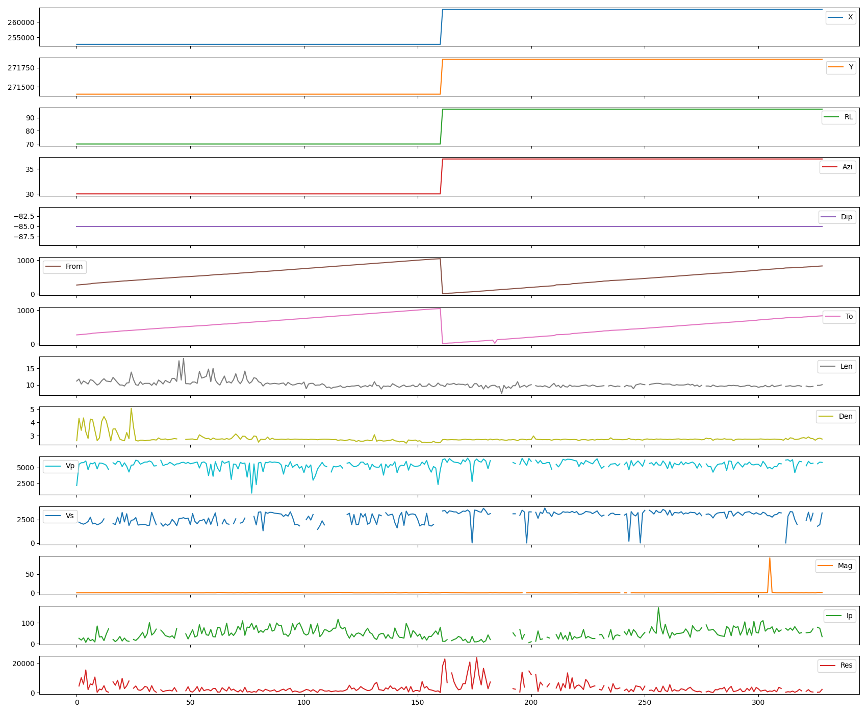
Among the variables in the dataset we have 4 texts (object) and 14 numeric variables (int64 and float64). The general behavior of the numerical variables can be seen in the following tables and graphs. Stand out the important anomaly in Mag, as well as the numerous missing values (NaN) in Vp, Vs, Ip, and Res:
Type of data in the dataset
df.info()
<class 'pandas.core.frame.DataFrame'>
RangeIndex: 329 entries, 0 to 328
Data columns (total 18 columns):
 #   Column  Non-Null Count  Dtype
---  ------  --------------  -----
 0   Hole    329 non-null    object
 1   X       329 non-null    float64
 2   Y       329 non-null    float64
 3   RL      329 non-null    float64
 4   Azi     329 non-null    int64
 5   Dip     329 non-null    int64
 6   Sample  329 non-null    object
 7   From    329 non-null    float64
 8   To      329 non-null    float64
 9   Len     321 non-null    float64
 10  Den     327 non-null    float64
 11  Vp      310 non-null    float64
 12  Vs      289 non-null    float64
 13  Mag     326 non-null    float64
 14  Ip      303 non-null    float64
 15  Res     303 non-null    float64
 16  Obs     73 non-null     object
 17  Form    329 non-null    object
dtypes: float64(12), int64(2), object(4)
memory usage: 46.4+ KB
NaN in Len
print('NaNs in Len:', 329 - 321)
NaNs in Len: 8
Main statistical parameters of the variables
df.describe()
All numerical variables in line plots, the x axis is just the position in the file.
df.plot(figsize=(17, 14), subplots=True)
plt.tight_layout()
# plt.savefig('Output/lines.png')
plt.show()
Null Values (NaN) in the Variables
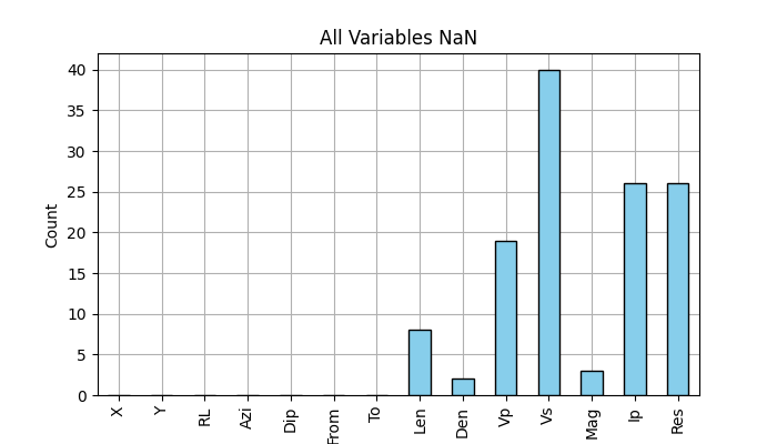
As can be seen in the previous cells and plots, most of the NaN are in Vp, Vs, Ip, and Re. Obs, a text variable, has also a lot (77.8%) of NaNs.
% of NaN in all variables
print('% of NaN in all variables:')
df.isna().sum()*100/len(df)
% of NaN in all variables:

Hole       0.000000
X          0.000000
Y          0.000000
RL         0.000000
Azi        0.000000
Dip        0.000000
Sample     0.000000
From       0.000000
To         0.000000
Len        2.431611
Den        0.607903
Vp         5.775076
Vs        12.158055
Mag        0.911854
Ip         7.902736
Res        7.902736
Obs       77.811550
Form       0.000000
dtype: float64
Plot of the number of NaN in the numerical variables
df.select_dtypes(include=['number']).isna().sum().plot.bar(figsize=(7, 4), ylabel='Count', edgecolor='k', color='skyblue', title='All Variables NaN', zorder=2)
plt.grid(zorder=1)
plt.show()
Reference Variables
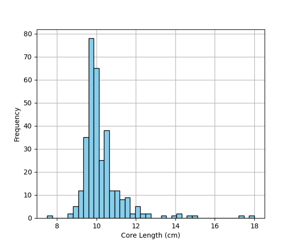
Not all numerical variables are suitable for modeling. In addition to the text variables (Hole, Sample, Obs, Form), X, Y, RL, Azi, Dip, From, To, and Len are reference or location variables. Among these, Len represents the length of the cores used for measurements, with an average length of 10.2 cm.
# Plot core length histogram
df.Len.plot.hist(figsize=(6, 5), subplots=True, bins=40, edgecolor='k', color='skyblue', zorder=2)
plt.grid(zorder=1)
plt.xlabel('Core Length (cm)')
plt.show()
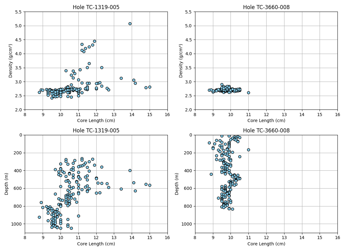
Core length influence on density
plt.figure(figsize=(11, 8))

plt.subplot(221)
plt.scatter(df.Len[df.Hole == 'TC-1319-005'], df.Den[df.Hole == 'TC-1319-005'], edgecolor='k', color='skyblue', zorder=2)
plt.grid(zorder=1)
plt.xlabel('Core Length (cm)')
plt.ylabel('Density (g/cm³)')
plt.axis([8, 16, 2, 5.5])
plt.title('Hole TC-1319-005')

plt.subplot(222)
plt.scatter(df.Len[df.Hole == 'TC-3660-008'], df.Den[df.Hole == 'TC-3660-008'], edgecolor='k', color='skyblue', zorder=2)
plt.grid(zorder=1)
plt.xlabel('Core Length (cm)')
plt.ylabel('Density (g/cm³)')
plt.title('Hole TC-3660-008')
plt.axis([8, 16, 2, 5.5])

plt.subplot(223)
plt.scatter(df.Len[df.Hole == 'TC-1319-005'], df.From[df.Hole == 'TC-1319-005'], edgecolor='k', color='skyblue', zorder=2)
plt.grid(zorder=1)
plt.xlabel('Core Length (cm)')
plt.ylabel('Depth (m)')
plt.axis([8, 16, 1100, 0])
plt.title('Hole TC-1319-005')

plt.subplot(224)
plt.scatter(df.Len[df.Hole == 'TC-3660-008'], df.From[df.Hole == 'TC-3660-008'], edgecolor='k', color='skyblue', zorder=2)
plt.grid(zorder=1)
plt.xlabel('Core Length (cm)')
plt.ylabel('Depth (m)')
plt.title('Hole TC-3660-008')
plt.axis([8, 16, 1100, 0])

plt.tight_layout()
plt.show()
Modelable Variables or Features
In the following section, we will review, through the main statistical parameters and plots, each of the features or variables suitable for modeling. The variable From, the sample’s top depth, could have a double meaning, as a reference and feature. Len is not for modeling, it is important because allows the assessment of the quality of the density.
features = df[['Hole', 'From', 'Len', 'Den', 'Vp', 'Vs', 'Mag', 'Ip', 'Res', 'Form']]
features
features.describe()
Boxplot of each feature
features.plot.box(subplots=True, grid=False, figsize=(12, 7), layout=(3, 4), flierprops={"marker": "."})
plt.tight_layout()
# plt.savefig('Output/histos.png')
plt.show()
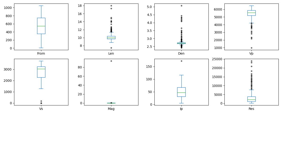
features.to_csv('Output/features.csv')
Density (Den)
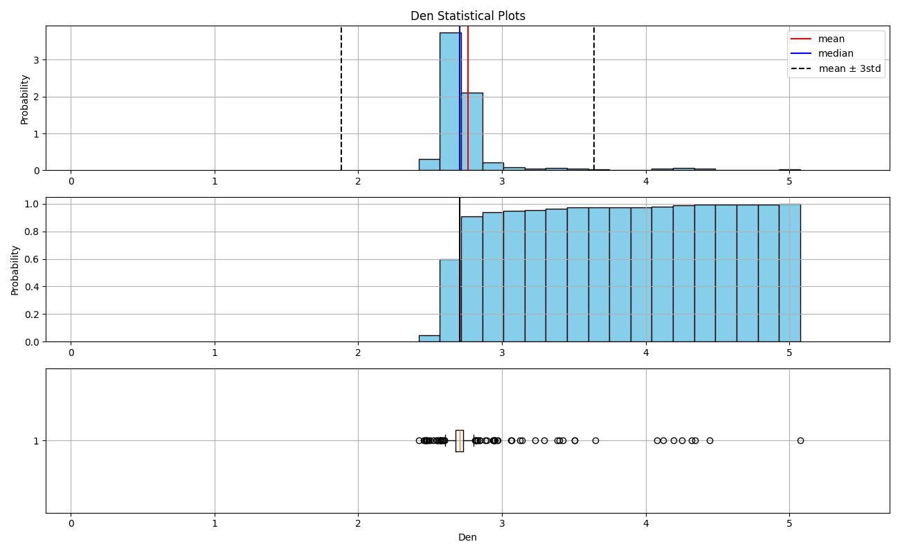
The distribution of the density variable has a wide tail to the right (positive skew), with anomalous values beyond +3 standard deviations. There is no mention, in the observations of the petrophysical data or in the stratigraphic logging of the hole, about the reason for these anomalous values, however, as it was seen previouly, the influence of long length (> 11.2 cm) in these high densities is clear.
Density statistical parameters by _aux
basic_stat.parameters(features.Den, 'Den')
---------------------------------------

Main statistical parameters of Den

NaN: 2
NaN(%): 0.608

Lenght: 329
Min: 2.42
Max: 5.074
Range: 2.654

Mean: 2.762
Median: 2.706
Mode: ModeResult(mode=np.float64(2.703), count=np.int64(9))

Mean < median: right tail
Skew: 4.618
Fisher's kurtosis: 24.334
Pearson's kurtosis: 27.334
Variance: 0.086
Standart deviation: 0.294
Mean - 3std: 1.880
Mean + 3std: 3.643
Density plots by _aux
basic_stat.plots(features.Den, 'Den')
8 observations with anomalous values in the density
features[features.Den > 4].sort_values(by='From')
Observations related to density
df[df.Den > 4].Obs
1                                             NaN
3                                             NaN
6                                             NaN
7                                             NaN
11                                            NaN
12                                            NaN
13                              Vs signal to low.
24    Sample too long to acquire IP measurements.
Name: Obs, dtype: object
den_anomalous_index = list(features[features.Den > 4].index)

print('Hole             Vp:        Observation:')
for n in den_anomalous_index:
    print(df.Hole[n], '    ', df.Den[n], '    ', df.Obs[n])
Hole             Vp:        Observation:
TC-1319-005      4.318      nan
TC-1319-005      4.342      nan
TC-1319-005      4.251      nan
TC-1319-005      4.193      nan
TC-1319-005      4.079      nan
TC-1319-005      4.444      nan
TC-1319-005      4.123      Vs signal to low.
TC-1319-005      5.074      Sample too long to acquire IP measurements.
Anomalies in Hole TC-1319-005
Apart from the fact that the anomalies are only in the TC-1319-005, there is almost no information related to the density anomalies. The stratigraphic logging mentioned abundant pyrite in hole TC-1319-005, around 1046 m, but this is far from the location of the anomalies in the petrophysical data (271.7 - 400.1 m).
Compressional Velocity (Vp)
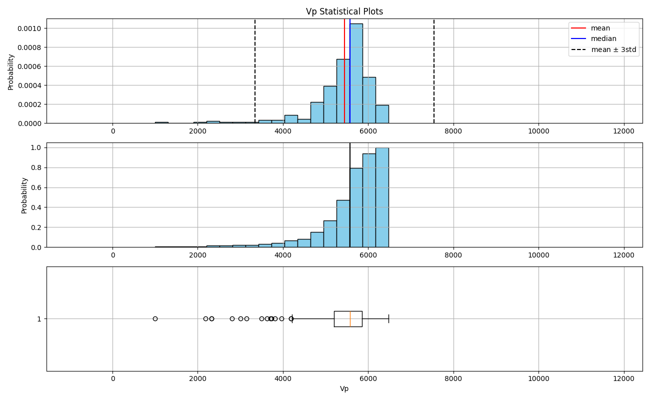
The distribution of the compressional velocity has a wide tail to the left (negative skew), with anomalous values below -3 standard deviations. The observations on these anomalous samples point toward open fractures on the core as responsible for the low Vp values.
Below are two reference values of Vp, at 20ºC (source: https://www.engineeringtoolbox.com/sound-speed-water-d_598.html):
Medium |
Vp (m/s) |
|---|---|
Fresh Water |
1480 |
Air |
343 |
Vp statistical parameters
basic_stat.parameters(features.Vp, 'Vp')
---------------------------------------

Main statistical parameters of Vp

NaN: 19
NaN(%): 5.775

Lenght: 329
Min: 992.0
Max: 6478.0
Range: 5486.0

Mean: 5441.990
Median: 5575.0
Mode: ModeResult(mode=np.float64(5575.0), count=np.int64(8))

Mean < median: left tail
Skew: -2.427
Fisher's kurtosis: 9.138
Pearson's kurtosis: 12.138
Variance: 491202.042
Standart deviation: 700.858
Mean - 3std: 3339.416
Mean + 3std: 7544.565
Vp plots
basic_stat.plots(features.Vp, 'Vp')
5 obsevations with anomalous values in the Vp
features[features.Vp < 3000]
Observations related to Vp
vp_anomalous_index = list(features[features.Vp < 3000].index)

print('Hole             Vp:        Observation:')
for n in vp_anomalous_index:
    print(df.Hole[n], '    ', df.Vp[n], '    ', df.Obs[n])
Hole             Vp:        Observation:
TC-1319-005      2179.0      Broken sample parallel to z-axis prevented to take IP and Vs measurements.
TC-1319-005      992.0      Broken sample parallel to z-axis prevented to take Vp and Vs measurements.
TC-1319-005      2321.0      nan
TC-1319-005      2325.0      The sample had an unflat base. Vs signal to low.
TC-3660-008      2802.0      Sample had a broken disk. Full length 10,4cm
The mayority of Vp anomalies are concentrate in the hole TC-1319-005 and they appear to be related with the geometry and fractures in the core sample. The stratigraphic logging has not direct mentions of the low Vp.
Shear Velocity (Vs)
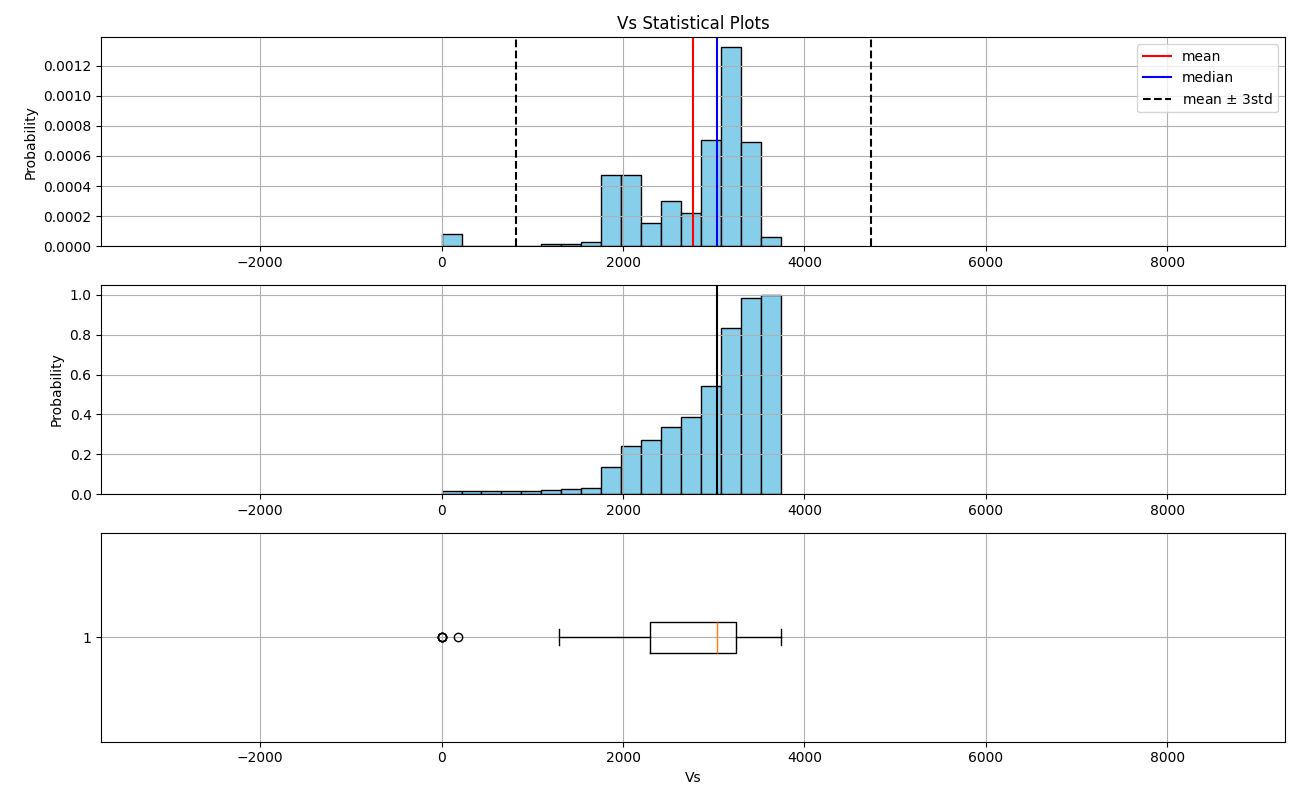
The distribution of the shear velocity has an irregular tail to the left (negative skew), with anomalous values below -3 standard deviations. As well as in the case of Vp, the observations on these anomalous values point toward open fractures on the core as responsible for the low Vs. Values of zero are not admissible in the case of solid samples, especially considering the densities in these anomalies (mean of 2.72). To improve subsequent models, these anomalous values of Vs should be replaced by NaN and then imputed (replaced by a logical value).
Below are two reference values of Vs (source: Reynolds, J (2011) An Introduction to Applied and Environmental Geophysics):
Medium |
Vs (m/s) |
|---|---|
Unconsolidated sands |
65-105 |
Plastic clays |
80-130 |
Vs statistical parameters
basic_stat.parameters(features.Vs, 'Vs')
---------------------------------------

Main statistical parameters of Vs

NaN: 40
NaN(%): 12.158

Lenght: 329
Min: 0.0
Max: 3740.0
Range: nan

Mean: 2772.938
Median: 3041.0
Mode: ModeResult(mode=np.float64(3333.0), count=np.int64(6))

Mean < median: left tail
Skew: -1.540
Fisher's kurtosis: 3.346
Pearson's kurtosis: 6.346
Variance: 426991.843
Standart deviation: 653.446
Mean - 3std: 812.599
Mean + 3std: 4733.276
Vp statistical parameterss plots
basic_stat.plots(features.Vs, 'Vs')
5 obsevations with anomalous values of Vs
features[features.Vs < 1000].sort_values(by='From')
Average density of the anomalous values of Vs
features[features.Vs < 1000].Den.mean()
np.float64(2.7216)
Observations related to Vs
vs_anomalous_index = list(features[features.Vs < 1000].index)

print('Hole             Vs:        Observation:')
for n in vs_anomalous_index:
    print(df.Hole[n], '    ', df.Vs[n], '    ', df.Obs[n])
Hole             Vs:        Observation:
TC-3660-008      0.0      Sample had a broken disk. Full length 10,4cm
TC-3660-008      0.0      Sample had unperpendicular bases respect from the z-axis that prevented to take IP measurements.
TC-3660-008      178.0      Chipped base
TC-3660-008      0.0      Chipped base
TC-3660-008      0.0      nan
Observations on Anomalies
Cllst_logging_details.xls has no mentions related to the zero Vs values. Other observations are:
Index |
Hole |
Reference Depth (m) |
Explanation |
|---|---|---|---|
175 |
TC-3660-008 |
64 |
|
198 & 311 | TC-3660-008 | 188 & 774 |
Diagenetic pyrite & pyrite in mudstones |
||
210 & 248 | TC-3660-008 | 432 & 452 |
Fault zone |
||
Once again, the majority of Vs anomalies are concentrated in the hole TC-1319-005 and they also appear to be related to fractures or the geometry of the core sample. The stratigraphic logging has no direct mentions of the low Vs.
Magnetic Susceptibility (Mag)
The magnetic susceptibility has an extremely anomalous value (93.89), which is 218 times higher than the average of the rest of the values (0.43). This outlier significantly skews the statistical parameters and visualizations, as it lies beyond 10 standard deviations above the mean. Removing this value reveals that the distribution has a tail to the right (positive skew), with some values exceeding 3 standard deviations.
Regarding the anomalous value, it exceeds the maximum value of 2 delivered by the KT-20 detector device, with a 10 kHz single-frequency circular sensor (https://terraplus.ca/wp-content/uploads/terraplus-Brochures-English/KT-20-Physical-Property-Measuring-System.pdf). Unfortunately, there are no specific observations that explain the reason for this extreme value.
Below are reference values of magnetic susceptibility for different rocks (source: https://www.eoas.ubc.ca/courses/eosc350/content/foundations/properties/magsuscept.htm#:~:text=In%20rocks%2C%20susceptibility%20is%20mainly,trace%20amounts%20in%20most%20sediments.):
Rock |
Magnetic Susceptibility x 10^-3 (SI) |
|---|---|
Limestones |
0 - 3 |
Sandstones |
0 - 20 |
Shales |
0.01 - 15 |
Gneiss |
0.1 - 25 |
Granite |
0 - 50 |
Basalt |
0.2 - 175 |
Magnetite |
1200 - 19200 |
Mag statistical parameters
basic_stat.parameters(features.Mag, 'Mag')
---------------------------------------

Main statistical parameters of Mag

NaN: 3
NaN(%): 0.912

Lenght: 329
Min: 0.001
Max: 93.886
Range: 93.88499999999999

Mean: 0.431
Median: 0.1145
Mode: ModeResult(mode=np.float64(0.063), count=np.int64(7))

Mean < median: right tail
Skew: 17.962
Fisher's kurtosis: 320.760
Pearson's kurtosis: 323.760
Variance: 26.966
Standart deviation: 5.193
Mean - 3std: -15.148
Mean + 3std: 16.009
Mag plots
basic_stat.plots(features.Mag, 'Mag')
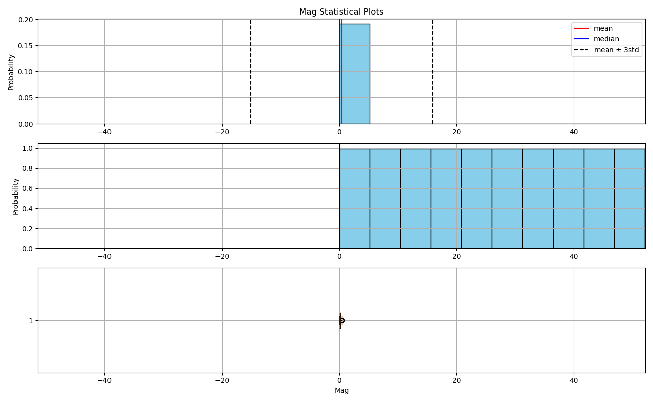
The maximum is 200 times bigger than the mean value
print('Index of the maximun:', features.Mag.idxmax())
print('Maximun value:', features.Mag[305])
Index of the maximun: 305
Maximun value: 93.886
features.loc[305]
Hole    TC-3660-008
From          734.8
Len             9.5
Den           2.708
Vp           5026.0
Vs           2914.0
Mag          93.886
Ip            71.63
Res          1200.0
Form             SP
Name: 305, dtype: object
Mag < 10 statistical parameters
basic_stat.parameters(features.Mag[features.Mag < 10], 'Mag')
---------------------------------------

Main statistical parameters of Mag

NaN: 0
NaN(%): 0.000

Lenght: 325
Min: 0.001
Max: 0.545
Range: 0.544

Mean: 0.143
Median: 0.114
Mode: ModeResult(mode=np.float64(0.063), count=np.int64(7))

Mean < median: right tail
Skew: 1.050
Fisher's kurtosis: 0.638
Pearson's kurtosis: 3.638
Variance: 0.010
Standart deviation: 0.101
Mean - 3std: -0.159
Mean + 3std: 0.445
Mag < 10 plots
basic_stat.plots(features.Mag[features.Mag < 10], 'Mag')
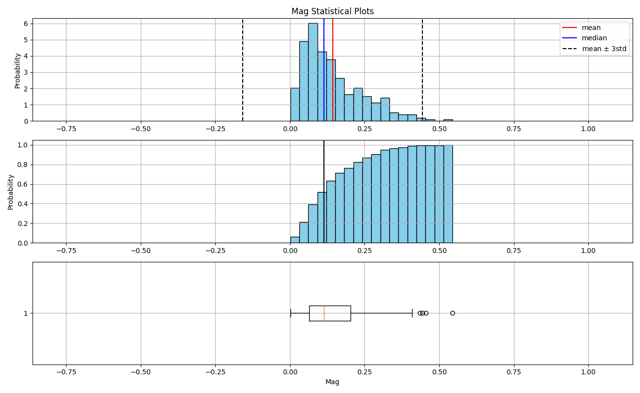
Mag anomalous value
df[df.Mag > 10]
The stratigraphic column mentions “pyrite in mudstones” in the interval corresponding to this sample but nothing related to tha Mag.
Induced Polarization (Ip)
Induced polarization or chargeability is the “capacity of a material to retain charges after a forcing current is removed.” It “depends upon many factors, including mineral type, grain size, the ratio of internal surface area to volume, the properties of electrolytes in pore space, and the physics of interaction between surfaces and fluids. Interpretation of chargeability models is further complicated by the fact that there is no standard set of units for this physical property.”(source: https://gpg.geosci.xyz/content/induced_polarization/induced_polarization_introduction.html). Ip is similar to conductivity (the inverse of resistivity) but not exactly the same, while the first is related with the capacitance of the material (retain electrical charges localized), the second is the ability of a material to allow the flow of electricity.
In our case, the measures of Ip have a tail to the right (positive skew), with only a value (171.73) above 3 standard deviations. There not observations associated with this value.
Ip statistical parameters
basic_stat.parameters(features.Ip, 'Ip')
---------------------------------------

Main statistical parameters of Ip

NaN: 26
NaN(%): 7.903

Lenght: 329
Min: 5.39
Max: 171.73
Range: nan

Mean: 49.739
Median: 47.04
Mode: ModeResult(mode=np.float64(7.27), count=np.int64(2))

Mean < median: right tail
Skew: 0.648
Fisher's kurtosis: 0.964
Pearson's kurtosis: 3.964
Variance: 632.281
Standart deviation: 25.145
Mean - 3std: -25.697
Mean + 3std: 125.174
Ip plots
basic_stat.plots(features.Ip, 'Ip')
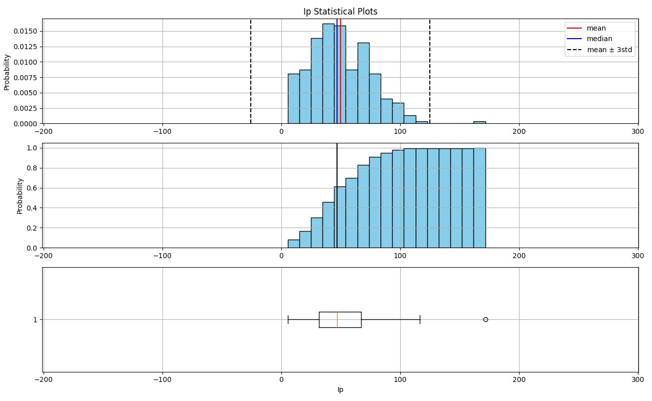
Ip anomalous value
df[df.Ip > 150]
No information about this anomaly in the petrophysical or in the stratigraphic data.
Resistivity (Res)
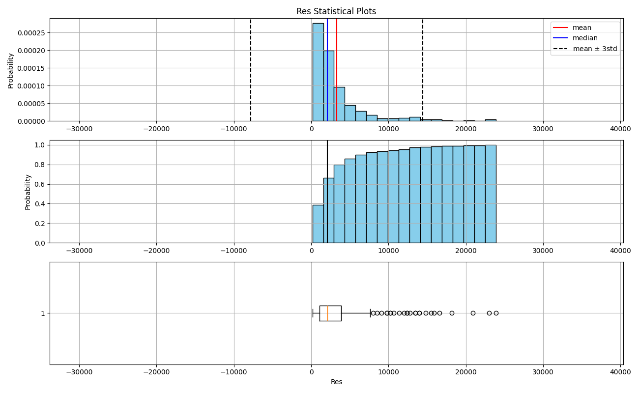
Although resistivity is a specific measure of pure materials, this property, like Ip, depends in the case of rocks on the constituent minerals and the fluids in their pore space. The measurements in our case show a typical pattern with tail to the right (positive skew) and with several values above 3 standard deviation. There are no observations associated with these high values.
Res statistical parameters
basic_stat.parameters(df.Res, 'Res')
---------------------------------------

Main statistical parameters of Res

NaN: 26
NaN(%): 7.903

Lenght: 329
Min: 156.9
Max: 23900.0
Range: nan

Mean: 3283.762
Median: 2100.0
Mode: ModeResult(mode=np.float64(1500.0), count=np.int64(12))

Mean < median: right tail
Skew: 2.729
Fisher's kurtosis: 8.783
Pearson's kurtosis: 11.783
Variance: 13800118.663
Standart deviation: 3714.851
Mean - 3std: -7860.791
Mean + 3std: 14428.316
Res plots
basic_stat.plots(df.Res, 'Res')
df[df.Res > 14000].sort_values(by='From')
Stratigraphic Data Observations ———————-_——– Only the stratigraphic data has observations of pyrite in hole TC-1319-005, but at shallower depths, around 146 & 193 m.
Features Correlation
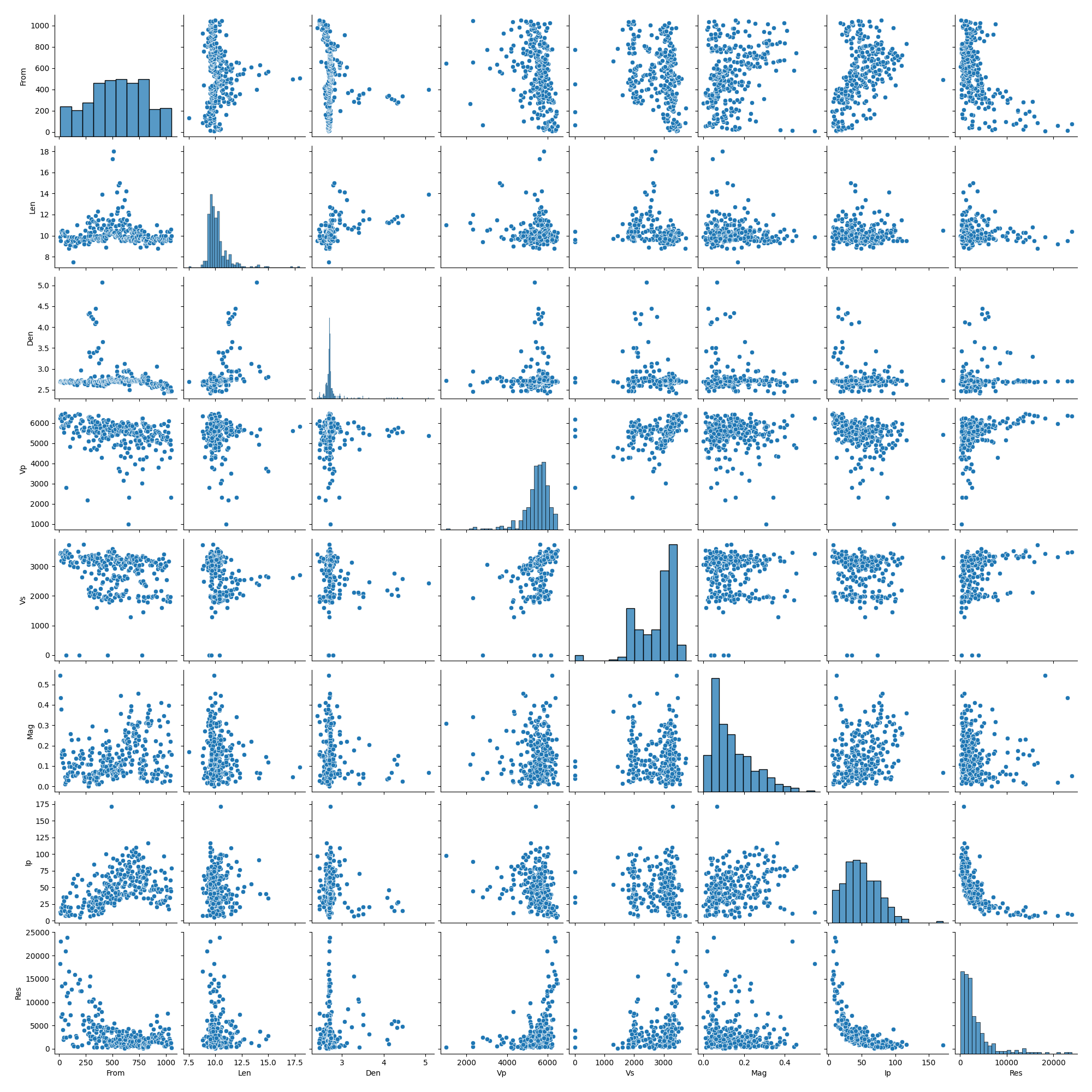
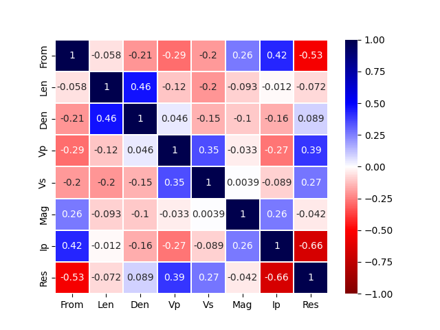
To appreciate the relation between the features, the anomaly of the Mag was excluded. No other elimination or imputation (fill with numbers the NaNs) was performed, therefore the quality of the correlations may change after the imputation.
# Pair Plot of All Features Against Each Other
mat = features[features.Mag < 10].select_dtypes(include=['number'])
sns.pairplot(mat)
plt.show()
Correlation Matrix
correl_mat = mat.corr()
correl_mat
Correlation Heatmap
sns.heatmap(correl_mat, vmin=-1, vmax=1, center=0, linewidths=.1, cmap='seismic_r', annot=True)
plt.show()
Additional Data Insights
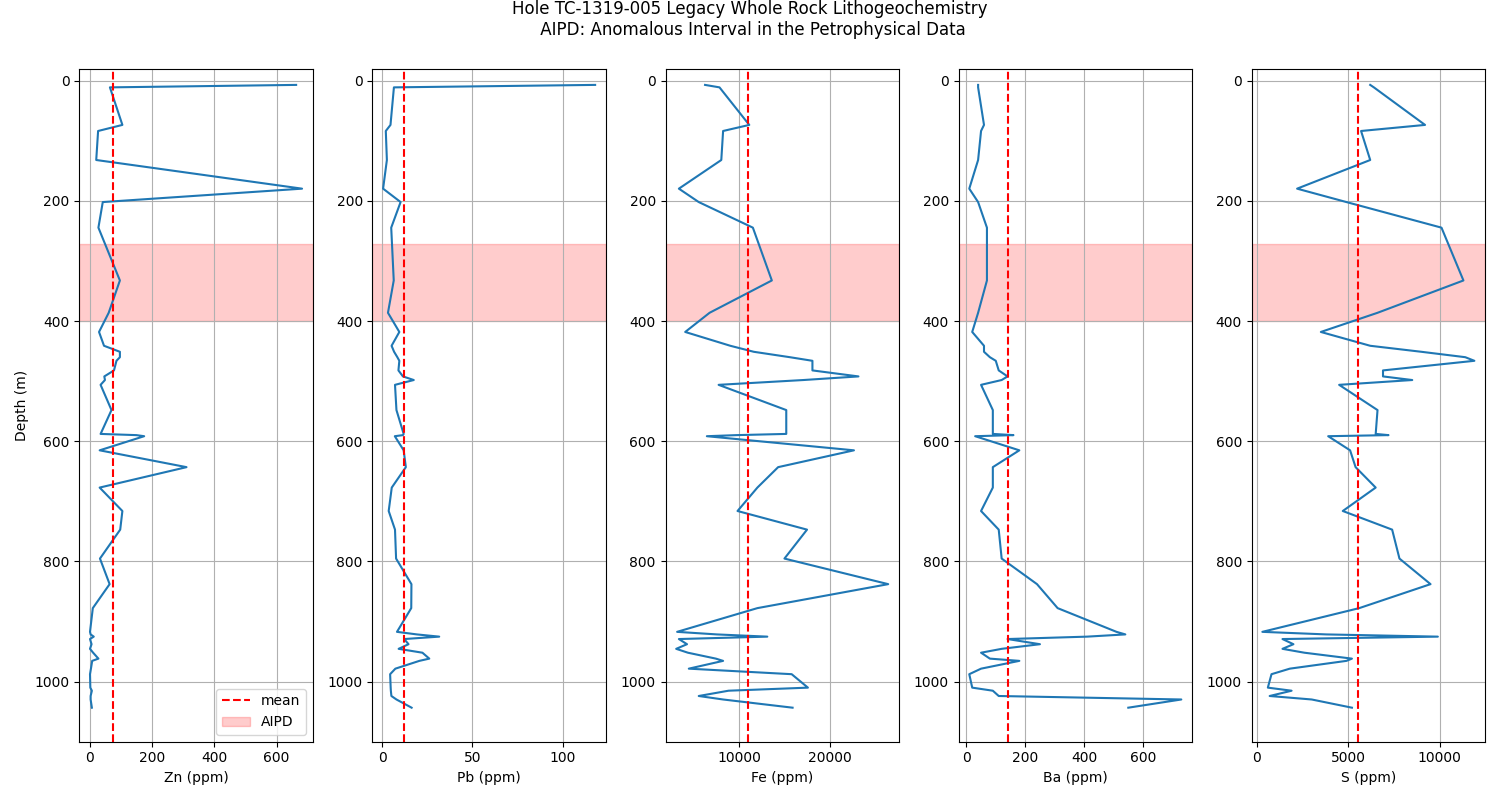
The main role of the additional datasets has been to help us understand the real nature of some anomalies observed in the petrophysical dataset, such as the density anomalies present in the upper half of the TC-1319-005 keyhole.
# Triple Plot by Major Formation
# Fix colors for the formations
import plotly.express as px
import plotly.io as pio

colors = px.colors.qualitative.Plotly

# Define color mapping for each formation
color_map = {form: colors[i % len(colors)] for i, form in enumerate(df['Form'].unique())}

# Set plot renderer and headless environment setup
pio.renderers.default = 'png'
pio.orca.config.use_xvfb = True

# 1x3 subplots
fig = make_subplots(
    rows=1, cols=3,
    subplot_titles=('Vp vs Den', 'Vp vs Vs', 'Vp/Vs vs Den')
)

# Plotting by formations
rat = df['Vp'] / df['Vs']

for form in df['Form'].unique():
    df_form = df[df['Form'] == form]
    rat_form = rat[df['Form'] == form]

    trace1 = go.Scatter(
        x=df_form['Vp'], y=df_form['Den'], mode='markers', name=form,
        legendgroup=form, marker=dict(color=color_map[form]),
        hovertext=df_form['Hole'],
        hoverinfo='x+y+text'
    )

    trace2 = go.Scatter(
        x=df_form['Vp'], y=df_form['Vs'], mode='markers', name=form,
        legendgroup=form, showlegend=False, marker=dict(color=color_map[form]),
        hovertext=df_form['Hole'],
        hoverinfo='x+y+text'
    )

    trace3 = go.Scatter(
        x=rat_form, y=df_form['Den'], mode='markers', name=form,
        legendgroup=form, showlegend=False, marker=dict(color=color_map[form]),
        hovertext=df_form['Hole'],
        hoverinfo='x+y+text'
    )

    fig.add_trace(trace1, row=1, col=1)
    fig.add_trace(trace2, row=1, col=2)
    fig.add_trace(trace3, row=1, col=3)

# Adjusting title and figure size
fig.update_layout(
    height=800,  # Figure height
    width=1600,  # Figure width
    title_text="Plots by Major Formations",
    showlegend=True,
    legend=dict(x=1.02, y=1)  # Adjust legend position
)
A module that was compiled using NumPy 1.x cannot be run in
NumPy 2.0.2 as it may crash. To support both 1.x and 2.x
versions of NumPy, modules must be compiled with NumPy 2.0.
Some module may need to rebuild instead e.g. with 'pybind11>=2.12'.

If you are a user of the module, the easiest solution will be to
downgrade to 'numpy<2' or try to upgrade the affected module.
We expect that some modules will need time to support NumPy 2.

Traceback (most recent call last):  File "/home/leguark/.virtualenvs/gempy_dependencies/bin/sphinx-build", line 8, in <module>
    sys.exit(main())
  File "/home/leguark/.virtualenvs/gempy_dependencies/lib/python3.10/site-packages/sphinx/cmd/build.py", line 339, in main
    return make_main(argv)
  File "/home/leguark/.virtualenvs/gempy_dependencies/lib/python3.10/site-packages/sphinx/cmd/build.py", line 213, in make_main
    return make_mode.run_make_mode(argv[1:])
  File "/home/leguark/.virtualenvs/gempy_dependencies/lib/python3.10/site-packages/sphinx/cmd/make_mode.py", line 181, in run_make_mode
    return make.run_generic_build(args[0])
  File "/home/leguark/.virtualenvs/gempy_dependencies/lib/python3.10/site-packages/sphinx/cmd/make_mode.py", line 169, in run_generic_build
    return build_main(args + opts)
  File "/home/leguark/.virtualenvs/gempy_dependencies/lib/python3.10/site-packages/sphinx/cmd/build.py", line 293, in build_main
    app = Sphinx(args.sourcedir, args.confdir, args.outputdir,
  File "/home/leguark/.virtualenvs/gempy_dependencies/lib/python3.10/site-packages/sphinx/application.py", line 272, in __init__
    self._init_builder()
  File "/home/leguark/.virtualenvs/gempy_dependencies/lib/python3.10/site-packages/sphinx/application.py", line 343, in _init_builder
    self.events.emit('builder-inited')
  File "/home/leguark/.virtualenvs/gempy_dependencies/lib/python3.10/site-packages/sphinx/events.py", line 97, in emit
    results.append(listener.handler(self.app, *args))
  File "/home/leguark/.virtualenvs/gempy_dependencies/lib/python3.10/site-packages/sphinx_gallery/gen_gallery.py", line 632, in generate_gallery_rst
    ) = generate_dir_rst(src_dir, target_dir, gallery_conf, seen_backrefs)
  File "/home/leguark/.virtualenvs/gempy_dependencies/lib/python3.10/site-packages/sphinx_gallery/gen_rst.py", line 531, in generate_dir_rst
    intro, title, (t, mem) = generate_file_rst(
  File "/home/leguark/.virtualenvs/gempy_dependencies/lib/python3.10/site-packages/sphinx_gallery/gen_rst.py", line 1203, in generate_file_rst
    output_blocks, time_elapsed = execute_script(
  File "/home/leguark/.virtualenvs/gempy_dependencies/lib/python3.10/site-packages/sphinx_gallery/gen_rst.py", line 1108, in execute_script
    execute_code_block(
  File "/home/leguark/.virtualenvs/gempy_dependencies/lib/python3.10/site-packages/sphinx_gallery/gen_rst.py", line 970, in execute_code_block
    is_last_expr, mem_max = _exec_and_get_memory(
  File "/home/leguark/.virtualenvs/gempy_dependencies/lib/python3.10/site-packages/sphinx_gallery/gen_rst.py", line 802, in _exec_and_get_memory
    mem_body, _ = gallery_conf["call_memory"](
  File "/home/leguark/.virtualenvs/gempy_dependencies/lib/python3.10/site-packages/sphinx_gallery/gen_gallery.py", line 244, in call_memory
    return 0.0, func()
  File "/home/leguark/.virtualenvs/gempy_dependencies/lib/python3.10/site-packages/sphinx_gallery/gen_rst.py", line 722, in __call__
    exec(self.code, self.fake_main.__dict__)
  File "/home/leguark/vector-geology/examples/05_petrophysics/01_eda_integration_delivery_1.py", line 551, in <module>
    import plotly.express as px
  File "/home/leguark/.virtualenvs/gempy_dependencies/lib/python3.10/site-packages/plotly/express/__init__.py", line 14, in <module>
    from ._imshow import imshow
  File "/home/leguark/.virtualenvs/gempy_dependencies/lib/python3.10/site-packages/plotly/express/_imshow.py", line 11, in <module>
    import xarray
  File "/home/leguark/.virtualenvs/gempy_dependencies/lib/python3.10/site-packages/xarray/__init__.py", line 3, in <module>
    from xarray import groupers, testing, tutorial
  File "/home/leguark/.virtualenvs/gempy_dependencies/lib/python3.10/site-packages/xarray/groupers.py", line 17, in <module>
    from xarray.coding.cftime_offsets import BaseCFTimeOffset, _new_to_legacy_freq
  File "/home/leguark/.virtualenvs/gempy_dependencies/lib/python3.10/site-packages/xarray/coding/cftime_offsets.py", line 56, in <module>
    from xarray.coding.cftimeindex import CFTimeIndex, _parse_iso8601_with_reso
  File "/home/leguark/.virtualenvs/gempy_dependencies/lib/python3.10/site-packages/xarray/coding/cftimeindex.py", line 54, in <module>
    from xarray.coding.times import (
  File "/home/leguark/.virtualenvs/gempy_dependencies/lib/python3.10/site-packages/xarray/coding/times.py", line 14, in <module>
    from xarray.coding.variables import (
  File "/home/leguark/.virtualenvs/gempy_dependencies/lib/python3.10/site-packages/xarray/coding/variables.py", line 13, in <module>
    from xarray.core import dtypes, duck_array_ops, indexing
  File "/home/leguark/.virtualenvs/gempy_dependencies/lib/python3.10/site-packages/xarray/core/indexing.py", line 20, in <module>
    from xarray.core.types import T_Xarray
  File "/home/leguark/.virtualenvs/gempy_dependencies/lib/python3.10/site-packages/xarray/core/types.py", line 106, in <module>
    from cftime import datetime as CFTimeDatetime
  File "/home/leguark/.virtualenvs/gempy_dependencies/lib/python3.10/site-packages/cftime/__init__.py", line 1, in <module>
    from ._cftime import (datetime, real_datetime,

A module that was compiled using NumPy 1.x cannot be run in
NumPy 2.0.2 as it may crash. To support both 1.x and 2.x
versions of NumPy, modules must be compiled with NumPy 2.0.
Some module may need to rebuild instead e.g. with 'pybind11>=2.12'.

If you are a user of the module, the easiest solution will be to
downgrade to 'numpy<2' or try to upgrade the affected module.
We expect that some modules will need time to support NumPy 2.

Traceback (most recent call last):  File "/home/leguark/.virtualenvs/gempy_dependencies/bin/sphinx-build", line 8, in <module>
    sys.exit(main())
  File "/home/leguark/.virtualenvs/gempy_dependencies/lib/python3.10/site-packages/sphinx/cmd/build.py", line 339, in main
    return make_main(argv)
  File "/home/leguark/.virtualenvs/gempy_dependencies/lib/python3.10/site-packages/sphinx/cmd/build.py", line 213, in make_main
    return make_mode.run_make_mode(argv[1:])
  File "/home/leguark/.virtualenvs/gempy_dependencies/lib/python3.10/site-packages/sphinx/cmd/make_mode.py", line 181, in run_make_mode
    return make.run_generic_build(args[0])
  File "/home/leguark/.virtualenvs/gempy_dependencies/lib/python3.10/site-packages/sphinx/cmd/make_mode.py", line 169, in run_generic_build
    return build_main(args + opts)
  File "/home/leguark/.virtualenvs/gempy_dependencies/lib/python3.10/site-packages/sphinx/cmd/build.py", line 293, in build_main
    app = Sphinx(args.sourcedir, args.confdir, args.outputdir,
  File "/home/leguark/.virtualenvs/gempy_dependencies/lib/python3.10/site-packages/sphinx/application.py", line 272, in __init__
    self._init_builder()
  File "/home/leguark/.virtualenvs/gempy_dependencies/lib/python3.10/site-packages/sphinx/application.py", line 343, in _init_builder
    self.events.emit('builder-inited')
  File "/home/leguark/.virtualenvs/gempy_dependencies/lib/python3.10/site-packages/sphinx/events.py", line 97, in emit
    results.append(listener.handler(self.app, *args))
  File "/home/leguark/.virtualenvs/gempy_dependencies/lib/python3.10/site-packages/sphinx_gallery/gen_gallery.py", line 632, in generate_gallery_rst
    ) = generate_dir_rst(src_dir, target_dir, gallery_conf, seen_backrefs)
  File "/home/leguark/.virtualenvs/gempy_dependencies/lib/python3.10/site-packages/sphinx_gallery/gen_rst.py", line 531, in generate_dir_rst
    intro, title, (t, mem) = generate_file_rst(
  File "/home/leguark/.virtualenvs/gempy_dependencies/lib/python3.10/site-packages/sphinx_gallery/gen_rst.py", line 1203, in generate_file_rst
    output_blocks, time_elapsed = execute_script(
  File "/home/leguark/.virtualenvs/gempy_dependencies/lib/python3.10/site-packages/sphinx_gallery/gen_rst.py", line 1108, in execute_script
    execute_code_block(
  File "/home/leguark/.virtualenvs/gempy_dependencies/lib/python3.10/site-packages/sphinx_gallery/gen_rst.py", line 970, in execute_code_block
    is_last_expr, mem_max = _exec_and_get_memory(
  File "/home/leguark/.virtualenvs/gempy_dependencies/lib/python3.10/site-packages/sphinx_gallery/gen_rst.py", line 802, in _exec_and_get_memory
    mem_body, _ = gallery_conf["call_memory"](
  File "/home/leguark/.virtualenvs/gempy_dependencies/lib/python3.10/site-packages/sphinx_gallery/gen_gallery.py", line 244, in call_memory
    return 0.0, func()
  File "/home/leguark/.virtualenvs/gempy_dependencies/lib/python3.10/site-packages/sphinx_gallery/gen_rst.py", line 722, in __call__
    exec(self.code, self.fake_main.__dict__)
  File "/home/leguark/vector-geology/examples/05_petrophysics/01_eda_integration_delivery_1.py", line 551, in <module>
    import plotly.express as px
  File "/home/leguark/.virtualenvs/gempy_dependencies/lib/python3.10/site-packages/plotly/express/__init__.py", line 14, in <module>
    from ._imshow import imshow
  File "/home/leguark/.virtualenvs/gempy_dependencies/lib/python3.10/site-packages/plotly/express/_imshow.py", line 11, in <module>
    import xarray
  File "/home/leguark/.virtualenvs/gempy_dependencies/lib/python3.10/site-packages/xarray/__init__.py", line 3, in <module>
    from xarray import groupers, testing, tutorial
  File "/home/leguark/.virtualenvs/gempy_dependencies/lib/python3.10/site-packages/xarray/groupers.py", line 17, in <module>
    from xarray.coding.cftime_offsets import BaseCFTimeOffset, _new_to_legacy_freq
  File "/home/leguark/.virtualenvs/gempy_dependencies/lib/python3.10/site-packages/xarray/coding/cftime_offsets.py", line 56, in <module>
    from xarray.coding.cftimeindex import CFTimeIndex, _parse_iso8601_with_reso
  File "/home/leguark/.virtualenvs/gempy_dependencies/lib/python3.10/site-packages/xarray/coding/cftimeindex.py", line 54, in <module>
    from xarray.coding.times import (
  File "/home/leguark/.virtualenvs/gempy_dependencies/lib/python3.10/site-packages/xarray/coding/times.py", line 14, in <module>
    from xarray.coding.variables import (
  File "/home/leguark/.virtualenvs/gempy_dependencies/lib/python3.10/site-packages/xarray/coding/variables.py", line 14, in <module>
    from xarray.core.variable import Variable
  File "/home/leguark/.virtualenvs/gempy_dependencies/lib/python3.10/site-packages/xarray/core/variable.py", line 20, in <module>
    from xarray.core import common, dtypes, duck_array_ops, indexing, nputils, ops, utils
  File "/home/leguark/.virtualenvs/gempy_dependencies/lib/python3.10/site-packages/xarray/core/common.py", line 28, in <module>
    import cftime
  File "/home/leguark/.virtualenvs/gempy_dependencies/lib/python3.10/site-packages/cftime/__init__.py", line 1, in <module>
    from ._cftime import (datetime, real_datetime,

A module that was compiled using NumPy 1.x cannot be run in
NumPy 2.0.2 as it may crash. To support both 1.x and 2.x
versions of NumPy, modules must be compiled with NumPy 2.0.
Some module may need to rebuild instead e.g. with 'pybind11>=2.12'.

If you are a user of the module, the easiest solution will be to
downgrade to 'numpy<2' or try to upgrade the affected module.
We expect that some modules will need time to support NumPy 2.

Traceback (most recent call last):  File "/home/leguark/.virtualenvs/gempy_dependencies/bin/sphinx-build", line 8, in <module>
    sys.exit(main())
  File "/home/leguark/.virtualenvs/gempy_dependencies/lib/python3.10/site-packages/sphinx/cmd/build.py", line 339, in main
    return make_main(argv)
  File "/home/leguark/.virtualenvs/gempy_dependencies/lib/python3.10/site-packages/sphinx/cmd/build.py", line 213, in make_main
    return make_mode.run_make_mode(argv[1:])
  File "/home/leguark/.virtualenvs/gempy_dependencies/lib/python3.10/site-packages/sphinx/cmd/make_mode.py", line 181, in run_make_mode
    return make.run_generic_build(args[0])
  File "/home/leguark/.virtualenvs/gempy_dependencies/lib/python3.10/site-packages/sphinx/cmd/make_mode.py", line 169, in run_generic_build
    return build_main(args + opts)
  File "/home/leguark/.virtualenvs/gempy_dependencies/lib/python3.10/site-packages/sphinx/cmd/build.py", line 293, in build_main
    app = Sphinx(args.sourcedir, args.confdir, args.outputdir,
  File "/home/leguark/.virtualenvs/gempy_dependencies/lib/python3.10/site-packages/sphinx/application.py", line 272, in __init__
    self._init_builder()
  File "/home/leguark/.virtualenvs/gempy_dependencies/lib/python3.10/site-packages/sphinx/application.py", line 343, in _init_builder
    self.events.emit('builder-inited')
  File "/home/leguark/.virtualenvs/gempy_dependencies/lib/python3.10/site-packages/sphinx/events.py", line 97, in emit
    results.append(listener.handler(self.app, *args))
  File "/home/leguark/.virtualenvs/gempy_dependencies/lib/python3.10/site-packages/sphinx_gallery/gen_gallery.py", line 632, in generate_gallery_rst
    ) = generate_dir_rst(src_dir, target_dir, gallery_conf, seen_backrefs)
  File "/home/leguark/.virtualenvs/gempy_dependencies/lib/python3.10/site-packages/sphinx_gallery/gen_rst.py", line 531, in generate_dir_rst
    intro, title, (t, mem) = generate_file_rst(
  File "/home/leguark/.virtualenvs/gempy_dependencies/lib/python3.10/site-packages/sphinx_gallery/gen_rst.py", line 1203, in generate_file_rst
    output_blocks, time_elapsed = execute_script(
  File "/home/leguark/.virtualenvs/gempy_dependencies/lib/python3.10/site-packages/sphinx_gallery/gen_rst.py", line 1108, in execute_script
    execute_code_block(
  File "/home/leguark/.virtualenvs/gempy_dependencies/lib/python3.10/site-packages/sphinx_gallery/gen_rst.py", line 970, in execute_code_block
    is_last_expr, mem_max = _exec_and_get_memory(
  File "/home/leguark/.virtualenvs/gempy_dependencies/lib/python3.10/site-packages/sphinx_gallery/gen_rst.py", line 802, in _exec_and_get_memory
    mem_body, _ = gallery_conf["call_memory"](
  File "/home/leguark/.virtualenvs/gempy_dependencies/lib/python3.10/site-packages/sphinx_gallery/gen_gallery.py", line 244, in call_memory
    return 0.0, func()
  File "/home/leguark/.virtualenvs/gempy_dependencies/lib/python3.10/site-packages/sphinx_gallery/gen_rst.py", line 722, in __call__
    exec(self.code, self.fake_main.__dict__)
  File "/home/leguark/vector-geology/examples/05_petrophysics/01_eda_integration_delivery_1.py", line 551, in <module>
    import plotly.express as px
  File "/home/leguark/.virtualenvs/gempy_dependencies/lib/python3.10/site-packages/plotly/express/__init__.py", line 14, in <module>
    from ._imshow import imshow
  File "/home/leguark/.virtualenvs/gempy_dependencies/lib/python3.10/site-packages/plotly/express/_imshow.py", line 11, in <module>
    import xarray
  File "/home/leguark/.virtualenvs/gempy_dependencies/lib/python3.10/site-packages/xarray/__init__.py", line 3, in <module>
    from xarray import groupers, testing, tutorial
  File "/home/leguark/.virtualenvs/gempy_dependencies/lib/python3.10/site-packages/xarray/groupers.py", line 17, in <module>
    from xarray.coding.cftime_offsets import BaseCFTimeOffset, _new_to_legacy_freq
  File "/home/leguark/.virtualenvs/gempy_dependencies/lib/python3.10/site-packages/xarray/coding/cftime_offsets.py", line 56, in <module>
    from xarray.coding.cftimeindex import CFTimeIndex, _parse_iso8601_with_reso
  File "/home/leguark/.virtualenvs/gempy_dependencies/lib/python3.10/site-packages/xarray/coding/cftimeindex.py", line 54, in <module>
    from xarray.coding.times import (
  File "/home/leguark/.virtualenvs/gempy_dependencies/lib/python3.10/site-packages/xarray/coding/times.py", line 35, in <module>
    import cftime
  File "/home/leguark/.virtualenvs/gempy_dependencies/lib/python3.10/site-packages/cftime/__init__.py", line 1, in <module>
    from ._cftime import (datetime, real_datetime,

A module that was compiled using NumPy 1.x cannot be run in
NumPy 2.0.2 as it may crash. To support both 1.x and 2.x
versions of NumPy, modules must be compiled with NumPy 2.0.
Some module may need to rebuild instead e.g. with 'pybind11>=2.12'.

If you are a user of the module, the easiest solution will be to
downgrade to 'numpy<2' or try to upgrade the affected module.
We expect that some modules will need time to support NumPy 2.

Traceback (most recent call last):  File "/home/leguark/.virtualenvs/gempy_dependencies/bin/sphinx-build", line 8, in <module>
    sys.exit(main())
  File "/home/leguark/.virtualenvs/gempy_dependencies/lib/python3.10/site-packages/sphinx/cmd/build.py", line 339, in main
    return make_main(argv)
  File "/home/leguark/.virtualenvs/gempy_dependencies/lib/python3.10/site-packages/sphinx/cmd/build.py", line 213, in make_main
    return make_mode.run_make_mode(argv[1:])
  File "/home/leguark/.virtualenvs/gempy_dependencies/lib/python3.10/site-packages/sphinx/cmd/make_mode.py", line 181, in run_make_mode
    return make.run_generic_build(args[0])
  File "/home/leguark/.virtualenvs/gempy_dependencies/lib/python3.10/site-packages/sphinx/cmd/make_mode.py", line 169, in run_generic_build
    return build_main(args + opts)
  File "/home/leguark/.virtualenvs/gempy_dependencies/lib/python3.10/site-packages/sphinx/cmd/build.py", line 293, in build_main
    app = Sphinx(args.sourcedir, args.confdir, args.outputdir,
  File "/home/leguark/.virtualenvs/gempy_dependencies/lib/python3.10/site-packages/sphinx/application.py", line 272, in __init__
    self._init_builder()
  File "/home/leguark/.virtualenvs/gempy_dependencies/lib/python3.10/site-packages/sphinx/application.py", line 343, in _init_builder
    self.events.emit('builder-inited')
  File "/home/leguark/.virtualenvs/gempy_dependencies/lib/python3.10/site-packages/sphinx/events.py", line 97, in emit
    results.append(listener.handler(self.app, *args))
  File "/home/leguark/.virtualenvs/gempy_dependencies/lib/python3.10/site-packages/sphinx_gallery/gen_gallery.py", line 632, in generate_gallery_rst
    ) = generate_dir_rst(src_dir, target_dir, gallery_conf, seen_backrefs)
  File "/home/leguark/.virtualenvs/gempy_dependencies/lib/python3.10/site-packages/sphinx_gallery/gen_rst.py", line 531, in generate_dir_rst
    intro, title, (t, mem) = generate_file_rst(
  File "/home/leguark/.virtualenvs/gempy_dependencies/lib/python3.10/site-packages/sphinx_gallery/gen_rst.py", line 1203, in generate_file_rst
    output_blocks, time_elapsed = execute_script(
  File "/home/leguark/.virtualenvs/gempy_dependencies/lib/python3.10/site-packages/sphinx_gallery/gen_rst.py", line 1108, in execute_script
    execute_code_block(
  File "/home/leguark/.virtualenvs/gempy_dependencies/lib/python3.10/site-packages/sphinx_gallery/gen_rst.py", line 970, in execute_code_block
    is_last_expr, mem_max = _exec_and_get_memory(
  File "/home/leguark/.virtualenvs/gempy_dependencies/lib/python3.10/site-packages/sphinx_gallery/gen_rst.py", line 802, in _exec_and_get_memory
    mem_body, _ = gallery_conf["call_memory"](
  File "/home/leguark/.virtualenvs/gempy_dependencies/lib/python3.10/site-packages/sphinx_gallery/gen_gallery.py", line 244, in call_memory
    return 0.0, func()
  File "/home/leguark/.virtualenvs/gempy_dependencies/lib/python3.10/site-packages/sphinx_gallery/gen_rst.py", line 722, in __call__
    exec(self.code, self.fake_main.__dict__)
  File "/home/leguark/vector-geology/examples/05_petrophysics/01_eda_integration_delivery_1.py", line 551, in <module>
    import plotly.express as px
  File "/home/leguark/.virtualenvs/gempy_dependencies/lib/python3.10/site-packages/plotly/express/__init__.py", line 14, in <module>
    from ._imshow import imshow
  File "/home/leguark/.virtualenvs/gempy_dependencies/lib/python3.10/site-packages/plotly/express/_imshow.py", line 11, in <module>
    import xarray
  File "/home/leguark/.virtualenvs/gempy_dependencies/lib/python3.10/site-packages/xarray/__init__.py", line 3, in <module>
    from xarray import groupers, testing, tutorial
  File "/home/leguark/.virtualenvs/gempy_dependencies/lib/python3.10/site-packages/xarray/groupers.py", line 17, in <module>
    from xarray.coding.cftime_offsets import BaseCFTimeOffset, _new_to_legacy_freq
  File "/home/leguark/.virtualenvs/gempy_dependencies/lib/python3.10/site-packages/xarray/coding/cftime_offsets.py", line 56, in <module>
    from xarray.coding.cftimeindex import CFTimeIndex, _parse_iso8601_with_reso
  File "/home/leguark/.virtualenvs/gempy_dependencies/lib/python3.10/site-packages/xarray/coding/cftimeindex.py", line 64, in <module>
    import cftime
  File "/home/leguark/.virtualenvs/gempy_dependencies/lib/python3.10/site-packages/cftime/__init__.py", line 1, in <module>
    from ._cftime import (datetime, real_datetime,

A module that was compiled using NumPy 1.x cannot be run in
NumPy 2.0.2 as it may crash. To support both 1.x and 2.x
versions of NumPy, modules must be compiled with NumPy 2.0.
Some module may need to rebuild instead e.g. with 'pybind11>=2.12'.

If you are a user of the module, the easiest solution will be to
downgrade to 'numpy<2' or try to upgrade the affected module.
We expect that some modules will need time to support NumPy 2.

Traceback (most recent call last):  File "/home/leguark/.virtualenvs/gempy_dependencies/bin/sphinx-build", line 8, in <module>
    sys.exit(main())
  File "/home/leguark/.virtualenvs/gempy_dependencies/lib/python3.10/site-packages/sphinx/cmd/build.py", line 339, in main
    return make_main(argv)
  File "/home/leguark/.virtualenvs/gempy_dependencies/lib/python3.10/site-packages/sphinx/cmd/build.py", line 213, in make_main
    return make_mode.run_make_mode(argv[1:])
  File "/home/leguark/.virtualenvs/gempy_dependencies/lib/python3.10/site-packages/sphinx/cmd/make_mode.py", line 181, in run_make_mode
    return make.run_generic_build(args[0])
  File "/home/leguark/.virtualenvs/gempy_dependencies/lib/python3.10/site-packages/sphinx/cmd/make_mode.py", line 169, in run_generic_build
    return build_main(args + opts)
  File "/home/leguark/.virtualenvs/gempy_dependencies/lib/python3.10/site-packages/sphinx/cmd/build.py", line 293, in build_main
    app = Sphinx(args.sourcedir, args.confdir, args.outputdir,
  File "/home/leguark/.virtualenvs/gempy_dependencies/lib/python3.10/site-packages/sphinx/application.py", line 272, in __init__
    self._init_builder()
  File "/home/leguark/.virtualenvs/gempy_dependencies/lib/python3.10/site-packages/sphinx/application.py", line 343, in _init_builder
    self.events.emit('builder-inited')
  File "/home/leguark/.virtualenvs/gempy_dependencies/lib/python3.10/site-packages/sphinx/events.py", line 97, in emit
    results.append(listener.handler(self.app, *args))
  File "/home/leguark/.virtualenvs/gempy_dependencies/lib/python3.10/site-packages/sphinx_gallery/gen_gallery.py", line 632, in generate_gallery_rst
    ) = generate_dir_rst(src_dir, target_dir, gallery_conf, seen_backrefs)
  File "/home/leguark/.virtualenvs/gempy_dependencies/lib/python3.10/site-packages/sphinx_gallery/gen_rst.py", line 531, in generate_dir_rst
    intro, title, (t, mem) = generate_file_rst(
  File "/home/leguark/.virtualenvs/gempy_dependencies/lib/python3.10/site-packages/sphinx_gallery/gen_rst.py", line 1203, in generate_file_rst
    output_blocks, time_elapsed = execute_script(
  File "/home/leguark/.virtualenvs/gempy_dependencies/lib/python3.10/site-packages/sphinx_gallery/gen_rst.py", line 1108, in execute_script
    execute_code_block(
  File "/home/leguark/.virtualenvs/gempy_dependencies/lib/python3.10/site-packages/sphinx_gallery/gen_rst.py", line 970, in execute_code_block
    is_last_expr, mem_max = _exec_and_get_memory(
  File "/home/leguark/.virtualenvs/gempy_dependencies/lib/python3.10/site-packages/sphinx_gallery/gen_rst.py", line 802, in _exec_and_get_memory
    mem_body, _ = gallery_conf["call_memory"](
  File "/home/leguark/.virtualenvs/gempy_dependencies/lib/python3.10/site-packages/sphinx_gallery/gen_gallery.py", line 244, in call_memory
    return 0.0, func()
  File "/home/leguark/.virtualenvs/gempy_dependencies/lib/python3.10/site-packages/sphinx_gallery/gen_rst.py", line 722, in __call__
    exec(self.code, self.fake_main.__dict__)
  File "/home/leguark/vector-geology/examples/05_petrophysics/01_eda_integration_delivery_1.py", line 551, in <module>
    import plotly.express as px
  File "/home/leguark/.virtualenvs/gempy_dependencies/lib/python3.10/site-packages/plotly/express/__init__.py", line 14, in <module>
    from ._imshow import imshow
  File "/home/leguark/.virtualenvs/gempy_dependencies/lib/python3.10/site-packages/plotly/express/_imshow.py", line 11, in <module>
    import xarray
  File "/home/leguark/.virtualenvs/gempy_dependencies/lib/python3.10/site-packages/xarray/__init__.py", line 3, in <module>
    from xarray import groupers, testing, tutorial
  File "/home/leguark/.virtualenvs/gempy_dependencies/lib/python3.10/site-packages/xarray/groupers.py", line 17, in <module>
    from xarray.coding.cftime_offsets import BaseCFTimeOffset, _new_to_legacy_freq
  File "/home/leguark/.virtualenvs/gempy_dependencies/lib/python3.10/site-packages/xarray/coding/cftime_offsets.py", line 73, in <module>
    import cftime
  File "/home/leguark/.virtualenvs/gempy_dependencies/lib/python3.10/site-packages/cftime/__init__.py", line 1, in <module>
    from ._cftime import (datetime, real_datetime,

A module that was compiled using NumPy 1.x cannot be run in
NumPy 2.0.2 as it may crash. To support both 1.x and 2.x
versions of NumPy, modules must be compiled with NumPy 2.0.
Some module may need to rebuild instead e.g. with 'pybind11>=2.12'.

If you are a user of the module, the easiest solution will be to
downgrade to 'numpy<2' or try to upgrade the affected module.
We expect that some modules will need time to support NumPy 2.

Traceback (most recent call last):  File "/home/leguark/.virtualenvs/gempy_dependencies/bin/sphinx-build", line 8, in <module>
    sys.exit(main())
  File "/home/leguark/.virtualenvs/gempy_dependencies/lib/python3.10/site-packages/sphinx/cmd/build.py", line 339, in main
    return make_main(argv)
  File "/home/leguark/.virtualenvs/gempy_dependencies/lib/python3.10/site-packages/sphinx/cmd/build.py", line 213, in make_main
    return make_mode.run_make_mode(argv[1:])
  File "/home/leguark/.virtualenvs/gempy_dependencies/lib/python3.10/site-packages/sphinx/cmd/make_mode.py", line 181, in run_make_mode
    return make.run_generic_build(args[0])
  File "/home/leguark/.virtualenvs/gempy_dependencies/lib/python3.10/site-packages/sphinx/cmd/make_mode.py", line 169, in run_generic_build
    return build_main(args + opts)
  File "/home/leguark/.virtualenvs/gempy_dependencies/lib/python3.10/site-packages/sphinx/cmd/build.py", line 293, in build_main
    app = Sphinx(args.sourcedir, args.confdir, args.outputdir,
  File "/home/leguark/.virtualenvs/gempy_dependencies/lib/python3.10/site-packages/sphinx/application.py", line 272, in __init__
    self._init_builder()
  File "/home/leguark/.virtualenvs/gempy_dependencies/lib/python3.10/site-packages/sphinx/application.py", line 343, in _init_builder
    self.events.emit('builder-inited')
  File "/home/leguark/.virtualenvs/gempy_dependencies/lib/python3.10/site-packages/sphinx/events.py", line 97, in emit
    results.append(listener.handler(self.app, *args))
  File "/home/leguark/.virtualenvs/gempy_dependencies/lib/python3.10/site-packages/sphinx_gallery/gen_gallery.py", line 632, in generate_gallery_rst
    ) = generate_dir_rst(src_dir, target_dir, gallery_conf, seen_backrefs)
  File "/home/leguark/.virtualenvs/gempy_dependencies/lib/python3.10/site-packages/sphinx_gallery/gen_rst.py", line 531, in generate_dir_rst
    intro, title, (t, mem) = generate_file_rst(
  File "/home/leguark/.virtualenvs/gempy_dependencies/lib/python3.10/site-packages/sphinx_gallery/gen_rst.py", line 1203, in generate_file_rst
    output_blocks, time_elapsed = execute_script(
  File "/home/leguark/.virtualenvs/gempy_dependencies/lib/python3.10/site-packages/sphinx_gallery/gen_rst.py", line 1108, in execute_script
    execute_code_block(
  File "/home/leguark/.virtualenvs/gempy_dependencies/lib/python3.10/site-packages/sphinx_gallery/gen_rst.py", line 970, in execute_code_block
    is_last_expr, mem_max = _exec_and_get_memory(
  File "/home/leguark/.virtualenvs/gempy_dependencies/lib/python3.10/site-packages/sphinx_gallery/gen_rst.py", line 802, in _exec_and_get_memory
    mem_body, _ = gallery_conf["call_memory"](
  File "/home/leguark/.virtualenvs/gempy_dependencies/lib/python3.10/site-packages/sphinx_gallery/gen_gallery.py", line 244, in call_memory
    return 0.0, func()
  File "/home/leguark/.virtualenvs/gempy_dependencies/lib/python3.10/site-packages/sphinx_gallery/gen_rst.py", line 722, in __call__
    exec(self.code, self.fake_main.__dict__)
  File "/home/leguark/vector-geology/examples/05_petrophysics/01_eda_integration_delivery_1.py", line 551, in <module>
    import plotly.express as px
  File "/home/leguark/.virtualenvs/gempy_dependencies/lib/python3.10/site-packages/plotly/express/__init__.py", line 14, in <module>
    from ._imshow import imshow
  File "/home/leguark/.virtualenvs/gempy_dependencies/lib/python3.10/site-packages/plotly/express/_imshow.py", line 11, in <module>
    import xarray
  File "/home/leguark/.virtualenvs/gempy_dependencies/lib/python3.10/site-packages/xarray/__init__.py", line 3, in <module>
    from xarray import groupers, testing, tutorial
  File "/home/leguark/.virtualenvs/gempy_dependencies/lib/python3.10/site-packages/xarray/groupers.py", line 20, in <module>
    from xarray.core.dataarray import DataArray
  File "/home/leguark/.virtualenvs/gempy_dependencies/lib/python3.10/site-packages/xarray/core/dataarray.py", line 29, in <module>
    from xarray.coding.calendar_ops import convert_calendar, interp_calendar
  File "/home/leguark/.virtualenvs/gempy_dependencies/lib/python3.10/site-packages/xarray/coding/calendar_ops.py", line 20, in <module>
    import cftime
  File "/home/leguark/.virtualenvs/gempy_dependencies/lib/python3.10/site-packages/cftime/__init__.py", line 1, in <module>
    from ._cftime import (datetime, real_datetime,

A module that was compiled using NumPy 1.x cannot be run in
NumPy 2.0.2 as it may crash. To support both 1.x and 2.x
versions of NumPy, modules must be compiled with NumPy 2.0.
Some module may need to rebuild instead e.g. with 'pybind11>=2.12'.

If you are a user of the module, the easiest solution will be to
downgrade to 'numpy<2' or try to upgrade the affected module.
We expect that some modules will need time to support NumPy 2.

Traceback (most recent call last):  File "/home/leguark/.virtualenvs/gempy_dependencies/bin/sphinx-build", line 8, in <module>
    sys.exit(main())
  File "/home/leguark/.virtualenvs/gempy_dependencies/lib/python3.10/site-packages/sphinx/cmd/build.py", line 339, in main
    return make_main(argv)
  File "/home/leguark/.virtualenvs/gempy_dependencies/lib/python3.10/site-packages/sphinx/cmd/build.py", line 213, in make_main
    return make_mode.run_make_mode(argv[1:])
  File "/home/leguark/.virtualenvs/gempy_dependencies/lib/python3.10/site-packages/sphinx/cmd/make_mode.py", line 181, in run_make_mode
    return make.run_generic_build(args[0])
  File "/home/leguark/.virtualenvs/gempy_dependencies/lib/python3.10/site-packages/sphinx/cmd/make_mode.py", line 169, in run_generic_build
    return build_main(args + opts)
  File "/home/leguark/.virtualenvs/gempy_dependencies/lib/python3.10/site-packages/sphinx/cmd/build.py", line 293, in build_main
    app = Sphinx(args.sourcedir, args.confdir, args.outputdir,
  File "/home/leguark/.virtualenvs/gempy_dependencies/lib/python3.10/site-packages/sphinx/application.py", line 272, in __init__
    self._init_builder()
  File "/home/leguark/.virtualenvs/gempy_dependencies/lib/python3.10/site-packages/sphinx/application.py", line 343, in _init_builder
    self.events.emit('builder-inited')
  File "/home/leguark/.virtualenvs/gempy_dependencies/lib/python3.10/site-packages/sphinx/events.py", line 97, in emit
    results.append(listener.handler(self.app, *args))
  File "/home/leguark/.virtualenvs/gempy_dependencies/lib/python3.10/site-packages/sphinx_gallery/gen_gallery.py", line 632, in generate_gallery_rst
    ) = generate_dir_rst(src_dir, target_dir, gallery_conf, seen_backrefs)
  File "/home/leguark/.virtualenvs/gempy_dependencies/lib/python3.10/site-packages/sphinx_gallery/gen_rst.py", line 531, in generate_dir_rst
    intro, title, (t, mem) = generate_file_rst(
  File "/home/leguark/.virtualenvs/gempy_dependencies/lib/python3.10/site-packages/sphinx_gallery/gen_rst.py", line 1203, in generate_file_rst
    output_blocks, time_elapsed = execute_script(
  File "/home/leguark/.virtualenvs/gempy_dependencies/lib/python3.10/site-packages/sphinx_gallery/gen_rst.py", line 1108, in execute_script
    execute_code_block(
  File "/home/leguark/.virtualenvs/gempy_dependencies/lib/python3.10/site-packages/sphinx_gallery/gen_rst.py", line 970, in execute_code_block
    is_last_expr, mem_max = _exec_and_get_memory(
  File "/home/leguark/.virtualenvs/gempy_dependencies/lib/python3.10/site-packages/sphinx_gallery/gen_rst.py", line 802, in _exec_and_get_memory
    mem_body, _ = gallery_conf["call_memory"](
  File "/home/leguark/.virtualenvs/gempy_dependencies/lib/python3.10/site-packages/sphinx_gallery/gen_gallery.py", line 244, in call_memory
    return 0.0, func()
  File "/home/leguark/.virtualenvs/gempy_dependencies/lib/python3.10/site-packages/sphinx_gallery/gen_rst.py", line 722, in __call__
    exec(self.code, self.fake_main.__dict__)
  File "/home/leguark/vector-geology/examples/05_petrophysics/01_eda_integration_delivery_1.py", line 551, in <module>
    import plotly.express as px
  File "/home/leguark/.virtualenvs/gempy_dependencies/lib/python3.10/site-packages/plotly/express/__init__.py", line 14, in <module>
    from ._imshow import imshow
  File "/home/leguark/.virtualenvs/gempy_dependencies/lib/python3.10/site-packages/plotly/express/_imshow.py", line 11, in <module>
    import xarray
  File "/home/leguark/.virtualenvs/gempy_dependencies/lib/python3.10/site-packages/xarray/__init__.py", line 3, in <module>
    from xarray import groupers, testing, tutorial
  File "/home/leguark/.virtualenvs/gempy_dependencies/lib/python3.10/site-packages/xarray/groupers.py", line 20, in <module>
    from xarray.core.dataarray import DataArray
  File "/home/leguark/.virtualenvs/gempy_dependencies/lib/python3.10/site-packages/xarray/core/dataarray.py", line 49, in <module>
    from xarray.core.dataset import Dataset
  File "/home/leguark/.virtualenvs/gempy_dependencies/lib/python3.10/site-packages/xarray/core/dataset.py", line 131, in <module>
    from xarray.plot.accessor import DatasetPlotAccessor
  File "/home/leguark/.virtualenvs/gempy_dependencies/lib/python3.10/site-packages/xarray/plot/__init__.py", line 10, in <module>
    from xarray.plot.dataarray_plot import (
  File "/home/leguark/.virtualenvs/gempy_dependencies/lib/python3.10/site-packages/xarray/plot/dataarray_plot.py", line 13, in <module>
    from xarray.plot.facetgrid import _easy_facetgrid
  File "/home/leguark/.virtualenvs/gempy_dependencies/lib/python3.10/site-packages/xarray/plot/facetgrid.py", line 13, in <module>
    from xarray.plot.utils import (
  File "/home/leguark/.virtualenvs/gempy_dependencies/lib/python3.10/site-packages/xarray/plot/utils.py", line 30, in <module>
    import cftime
  File "/home/leguark/.virtualenvs/gempy_dependencies/lib/python3.10/site-packages/cftime/__init__.py", line 1, in <module>
    from ._cftime import (datetime, real_datetime,
Legacy Data Analysis
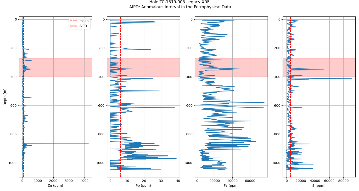
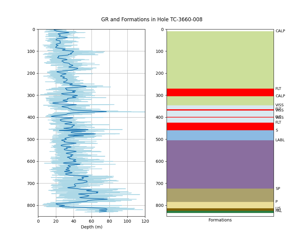
Legacy data played a crucial role in evaluating the density anomalies present in the keyhole TC-1319-005.
# Whole Rock Lithogeochemistry Data Load
whole = pd.read_csv(
    filepath_or_buffer=f'{base_path}/collinstown_wholerock_lithogeochemistry.csv',
    sep=';'
)
Renaming Columns and Filtering Data
whole = whole.rename(columns={'HOLEID'     : 'Hole', 'SAMPFROM': 'From', 'Zn_ppm_BEST': 'Zn',
                              'Pb_ppm_BEST': 'Pb', 'Ba_ppm_BEST': 'Ba', 'Fe_pct_BEST': 'Fe_pct',
                              'S_pct_BEST' : 'S_pct'})

# Convert % to ppm for Fe and S
whole['Fe'] = whole['Fe_pct'] * 10000
whole['S'] = whole['S_pct'] * 10000

# Drop unnecessary columns
whole = whole.drop(['Fe_pct', 'S_pct'], axis=1)

# Sort filtered data by "From"
whole5 = whole[whole.Hole == 'TC-1319-005'].sort_values('From')
Whole Rock Lithogeochemistry Plots
plt.figure(figsize=(15, 8))

# Plotting key elements
elem_list = ['Zn', 'Pb', 'Fe', 'Ba', 'S']

for element in elem_list:
    plt.subplot(1, 5, (elem_list.index(element) + 1))
    plt.plot(whole5[element], whole5.From)
    plt.axvline(x=np.mean(whole5[element]), ls='--', c='r', label='mean')
    plt.axhspan(272, 400, color='r', alpha=0.2, label='AIPD')
    plt.ylim(1100, -20)
    if elem_list.index(element) == 0:
        plt.ylabel('Depth (m)')
        plt.legend()
    plt.xlabel(f'{element} (ppm)')
    plt.grid()

plt.suptitle('Hole TC-1319-005 Legacy Whole Rock Lithogeochemistry\n AIPD: Anomalous Interval in the Petrophysical Data', y=1)
plt.tight_layout()
plt.show()
Legacy XRF data load
xrf = pd.read_csv(f'{base_path}/collinstown_pXRF.csv')
xrf.head()
xrf columns
xrf.columns
Index(['SAMPLEID', 'HOLEID', 'PROJECTCODE', 'SAMPFROM', 'SAMPTO', 'SAMPLETYPE',
       'FormationMaj_dr', 'FormationMin_dr', 'LithologyMaj_dr',
       'LithologyMin_dr', 'pXRF_Date', 'pXRF_ElapsedTime1',
       'pXRF_ElapsedTime2', 'pXRF_ElapsedTime3', 'pXRF_ElapsedTotalTim',
       'pXRF_InstrumentSN', 'pXRF_LiveTime1', 'pXRF_LiveTime2',
       'pXRF_LiveTime3', 'pXRF_LiveTotalTime', 'pXRF_Sampler', 'Reading',
       'X_Drillhole_dr', 'Y_Drillhole_dr', 'Z_Drillhole_dr', 'Ag_pXRF_pct',
       'Al_pXRF_pct', 'As_pXRF_pct', 'Bi_pXRF_pct', 'Ca_pXRF_pct',
       'Cd_pXRF_pct', 'Co_pXRF_pct', 'Cr_pXRF_pct', 'Cu_pXRF_pct',
       'Fe_pXRF_pct', 'Hg_pXRF_pct', 'K_pXRF_pct', 'LE_pXRF_pct',
       'Mg_pXRF_pct', 'Mn_pXRF_pct', 'Mo_pXRF_pct', 'Nb_pXRF_pct',
       'Ni_pXRF_pct', 'P_pXRF_pct', 'Pb_pXRF_pct', 'Rb_pXRF_pct', 'S_pXRF_pct',
       'Sb_pXRF_pct', 'Se_pXRF_pct', 'Si_pXRF_pct', 'Sn_pXRF_pct',
       'Sr_pXRF_pct', 'Th_pXRF_pct', 'Ti_pXRF_pct', 'U_pXRF_pct', 'V_pXRF_pct',
       'W_pXRF_pct', 'Y_pXRF_pct', 'Zn_pXRF_pct', 'Zr_pXRF_pct', 'PL_dr',
       'Sample_Dolomite1_Percent_dr', 'SampleComments_Big', 'Texture1_dr',
       'Texture2_dr', 'Texture3_dr'],
      dtype='object')
Main columns in xrf df
xrf = xrf[['HOLEID', 'SAMPFROM', 'Fe_pXRF_pct', 'Zn_pXRF_pct', 'Pb_pXRF_pct', 'S_pXRF_pct']]
xrf.head()
Conversion of % to ppm
columns_to_multiply = ['Fe_pXRF_pct', 'Zn_pXRF_pct', 'Pb_pXRF_pct', 'S_pXRF_pct']
xrf[columns_to_multiply] = xrf[columns_to_multiply] * 10000
xrf.head()
Rename the xrf columns
xrf = xrf.rename(columns={'HOLEID': 'Hole', 'SAMPFROM': 'From', 'Fe_pXRF_pct': 'Fe', 'Zn_pXRF_pct': 'Zn', 'Pb_pXRF_pct': 'Pb', 'S_pXRF_pct': 'S'})
xrf.head()
Sort by From
xrf5 = xrf[xrf.Hole == 'TC-1319-005'].sort_values('From')
xrf5.head()
Upper portion of xrf5
xrf5[xrf5.From <= 400].describe()
Elements in xrf5
elem_list2 = ['Zn', 'Pb', 'Fe', 'S']
XRF plots
plt.figure(figsize=(15, 8))

for element in elem_list2:
    plt.subplot(1, 4, (elem_list2.index(element) + 1))
    plt.plot(xrf5[element], xrf5.From)
    plt.axvline(x=np.mean(xrf5[element]), ls='--', c='r', label='mean')
    # plt.scatter(xrf5[element][200], xrf5.From[200], label='DPAL', c='k', zorder=3)
    plt.axhspan(272, 400, color='r', alpha=0.2, label='AIPD')
    plt.ylim(1100, -20)
    if elem_list.index(element) == 0:
        plt.ylabel('Depth (m)')
        plt.legend()
    plt.xlabel(f'{element} (ppm)')
    plt.grid()

plt.suptitle('Hole TC-1319-005 Legacy XRF\n AIPD: Anomalous Interval in the Petrophysical Data', y=1)
plt.tight_layout()
# plt.savefig('Output/xrf.png')
plt.show()
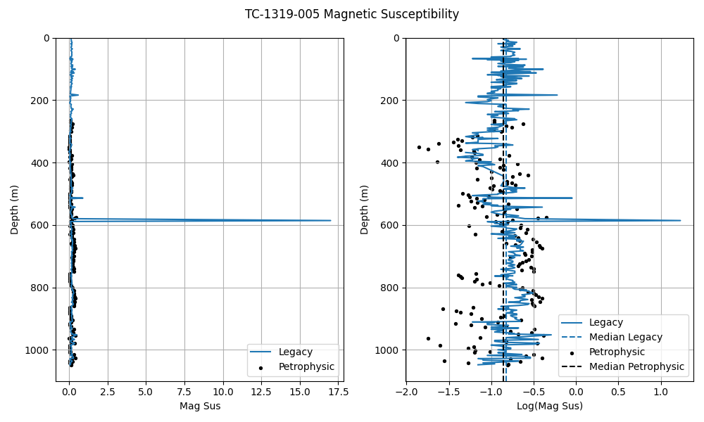
Magnetic Susceptibility
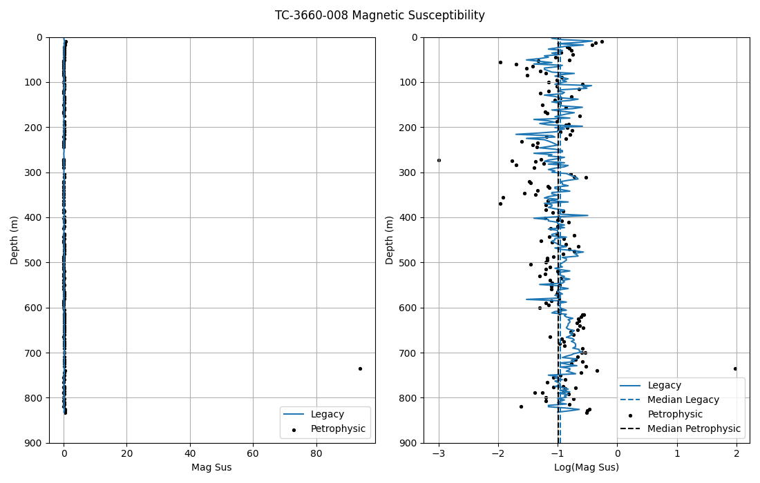
This section compares the magnetic susceptibility in the legacy and the latest petrophysical data. In the case of hole TC-1319-005 we can see that the magnetic susceptibility in both measurements have very similar medians. The magnetic susceptibilities, new and legacy, of hole TC-3660-008 have the same medians, but it has an anomaly in the petrophysical data that is above the measurement limit of the KT-20 device (2000 x $10^3$ SI), therefore this anomalous value is going to be deleted. Load magnetic susceptibility data
mag = pd.read_excel(f'{base_path}/collinstown_MagSUS.xlsx')
Magnetic Susceptibility Analysis for Hole TC-1319-005
mag5 = mag[mag.HOLEID == 'TC-1319-005'].sort_values('SAMPFROM')
petro5 = df[df.Hole == 'TC-1319-005'].sort_values('From')

plt.figure(figsize=(10, 6))

plt.subplot(121)
plt.plot(mag5['MS_MagSus'], mag5['SAMPFROM'], label='Legacy')
plt.scatter(petro5['Mag'], petro5['From'], c='k', label='Petrophysic', s=8)
plt.ylim(1100, 0)
plt.legend(loc='lower right')
plt.xlabel('Mag Sus')
plt.ylabel('Depth (m)')
plt.grid()

plt.subplot(122)
plt.plot(np.log10(mag5['MS_MagSus']), mag5['SAMPFROM'], label='Legacy')
plt.axvline(x=np.median(np.log10(mag5['MS_MagSus'])), ls='--', label='Median Legacy')
plt.scatter(np.log10(petro5['Mag']), petro5['From'], c='k', label='Petrophysic', s=8)
plt.axvline(x=np.median(np.log10(petro5['Mag'])), ls='--', c='k', label='Median Petrophysic')

plt.ylim(1100, 0)
plt.legend(loc='lower right')
plt.xlabel('Log(Mag Sus)')
plt.ylabel('Depth (m)')
plt.grid()

plt.suptitle('TC-1319-005 Magnetic Susceptibility')
plt.tight_layout()
plt.show()
Magnetic Susceptibility Analysis for Hole TC-3660-008
mag8 = mag[mag.HOLEID == 'TC-3660-008'].sort_values('SAMPFROM')
petro8 = df[df.Hole == 'TC-3660-008'].sort_values('From')

plt.figure(figsize=(11, 7))

plt.subplot(121)
plt.plot(mag8['MS_MagSus'], mag8['SAMPFROM'], label='Legacy')
plt.scatter(petro8['Mag'], petro8['From'], c='k', label='Petrophysic', s=8)
plt.ylim(900, 0)
plt.xlabel('Mag Sus')
plt.ylabel('Depth (m)')
plt.legend(loc='lower right')
plt.grid()

plt.subplot(122)
plt.plot(np.log10(mag8['MS_MagSus']), mag8['SAMPFROM'], label='Legacy')
plt.axvline(x=np.median(np.log10(mag8['MS_MagSus'])), ls='--', label='Median Legacy')
plt.scatter(np.log10(petro8['Mag']), petro8['From'], c='k', label='Petrophysic', s=8)
plt.axvline(x=np.nanmedian(np.log10(petro8['Mag'])), ls='--', c='k', label='Median Petrophysic')

plt.ylim(900, 0)
plt.xlabel('Log(Mag Sus)')
plt.ylabel('Depth (m)')
plt.legend(loc='lower right')
plt.grid()

plt.suptitle('TC-3660-008 Magnetic Susceptibility')
plt.tight_layout()
plt.show()
Gamma Ray and Formation Analysis for Hole TC-3660-008
gr = pd.read_csv(f'{base_path}/collinstown_Gamma.csv')
gr8 = gr[gr.HOLEID == 'TC-3660-008'].sort_values('DEPTH')

# Depth of tops or markers for formations
tops = pd.DataFrame(petro8.From[petro8['Form'].ne(petro8['Form'].shift())])
tops['Top'] = petro8.Form[petro8['Form'].ne(petro8['Form'].shift())]
tops = tops.reset_index(drop=True)

# Colors of the formations
tops['color'] = pd.Series(['#CCDF9A', '#FF0000', '#CCDF9A', '#D9E9F0', '#FF0000', '#D9E9F0', '#FF0000', '#D9E9F0', '#FF0000', '#8CBAE2',
                           '#8A6E9F', '#ABA16C', '#EBDE98', '#806000', '#2A7C43', '#FF0000'])

# Add base of the deepest formation
new_row = pd.DataFrame([{'From': 833.4, 'Top': '', 'color': '#FF0000'}])
tops = pd.concat([tops, new_row], ignore_index=True)
tops = tops.rename(columns={'From': 'depth', 'Top': 'name'})

tops_list = geo.plot_tops(tops)

gr8 = gr8.sort_values('DEPTH')
# Plot of GR with Formations

plt.figure(figsize=(10, 8))

plt.subplot(121)
plt.plot(gr8.iloc[:,6], gr8.iloc[:,5], label='Data', c='lightblue')
# plt.plot(gr8.iloc[:,6].rolling(window=250).mean(), gr8.iloc[:,5], label='Mean 400')

# Butterworth filter
b, a = butter(N=2, Wn=0.02, btype='low')
filtered_data = filtfilt(b, a, gr8.iloc[:, 6])
plt.plot(filtered_data, gr8.iloc[:, 5], label='Butterworth Filtered')

plt.grid()
plt.xlabel('GR (API)')
plt.xlabel('Depth (m)')
plt.axis([0, 120, 850, 0])

plt.subplot(122)
for i in range(0, len(tops_list)):
    plt.axhspan(tops_list[i]['top'], tops_list[i]['base'], color=tops_list[i]['color'])
    plt.text(122, tops_list[i]['top'], tops_list[i]['name'], fontsize=9, va='center')
plt.axis([0, 120, 850, 0])
plt.xticks([])
plt.xlabel('Formations')

plt.suptitle('GR and Formations in Hole TC-3660-008', y=0.93)
plt.savefig('Output/gr_form.png')
plt.show()
Passive Vs
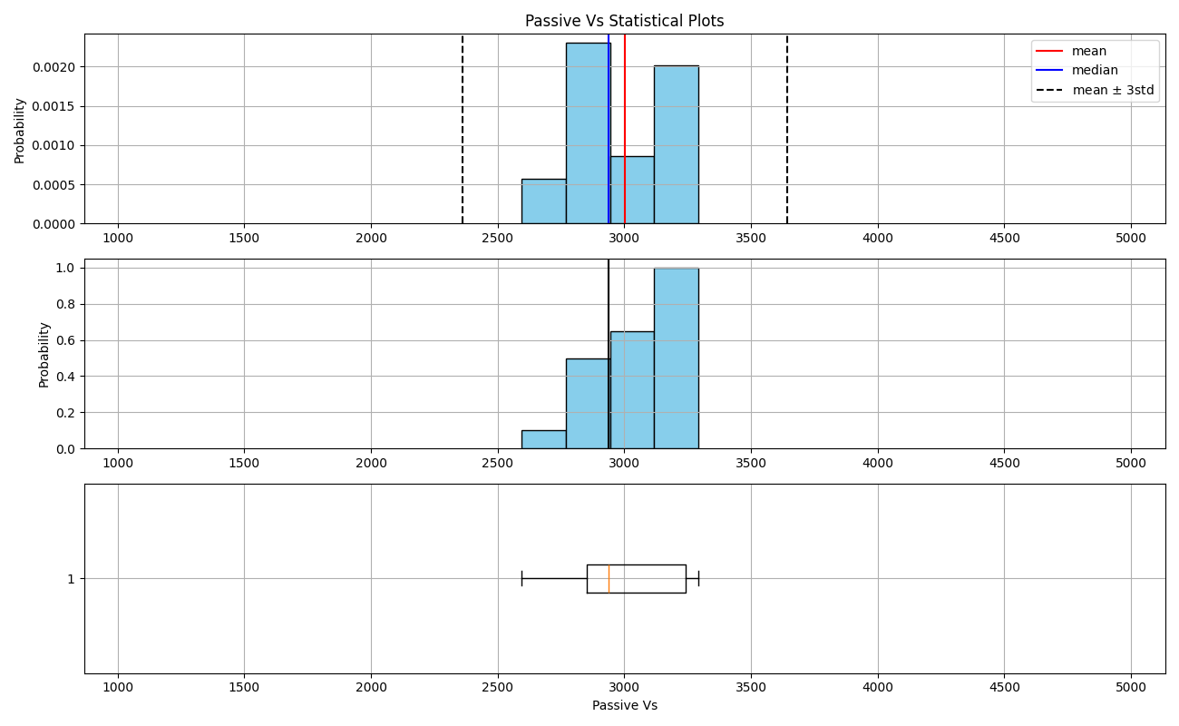
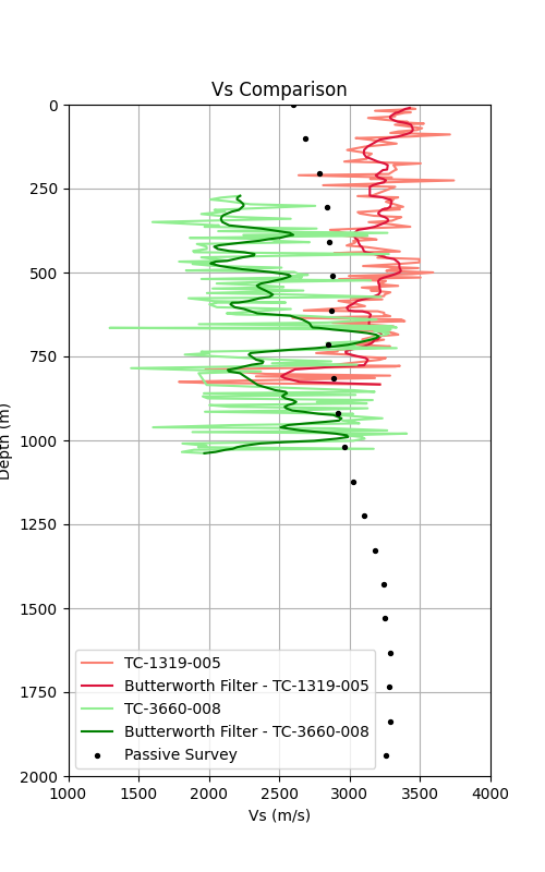
Parallel to the petrophysical measurements, a passive seismic survey was carried out between Collinstown and Kells. From this survey a Vs was obtained which can be compared with that recorded during the petrophysical measurements. Despite being measurements of a very different nature, the Vs of the key holes are in the range of values of the passive Vs. Refering to the trends, hole TC-1319-005, inside the survey, shows a contrary trend as the passive Vs. Paradoxically, Hole TC-3660-008, outside the survey, shows a trend that coincides with that of the passive Vs.
Load passive Vs data for hole TC-3660-008
pas = pd.read_csv(
    filepath_or_buffer=f'{base_path}/tc-3660-008_Vs.txt',
    sep=' ',
    skiprows=1,
    names=['depth_km', 'vs_km/s']
)

# Convert depth and velocity from km to m
pas[['depth_km', 'vs_km/s']] = pas[['depth_km', 'vs_km/s']] * 1000

# Rename columns for easier access
pas = pas.rename(columns={'depth_km': 'depth', 'vs_km/s': 'vs'})
Passive Vs Statistical Parameters
print(f"Basic statistics for Passive Vs:\n{pas['vs'].describe()}")
Basic statistics for Passive Vs:
count      20.000000
mean     3001.458200
std       219.007636
min      2595.905000
25%      2851.969250
50%      2937.861000
75%      3241.223000
max      3291.111000
Name: vs, dtype: float64
Passive Vs Plots
basic_stat.plots(pas.vs, 'Passive Vs')
Vs Comparison Plot
plt.figure(figsize=(5, 8))

# Vs at TC-1319-005
plt.plot(petro8.Vs[petro8.Vs >= 1000], petro8.From[petro8.Vs >= 1000], label='TC-1319-005', c='salmon')

# Apply Butterworth filter to TC-1319-005 Vs
b, a = butter(N=2, Wn=0.2, btype='low')
vs_butter = filtfilt(b, a, petro8.Vs[petro8.Vs >= 1000])
plt.plot(
    vs_butter,
    petro8.From[petro8.Vs >= 1000],
    label='Butterworth Filter - TC-1319-005',
    c='crimson'
)

# Vs at TC-3660-008
plt.plot(petro5.Vs[petro5.Vs >= 1000], petro5.From[petro5.Vs >= 1000], label='TC-3660-008', c='lightgreen')

# Apply Butterworth filter to TC-3660-008 Vs
vs_butter = filtfilt(b, a, petro5.Vs[petro5.Vs >= 1000])
plt.plot(
    vs_butter,
    petro5.From[petro5.Vs >= 1000],
    label='Butterworth Filter - TC-3660-008',
    c='green'
)

# Passive seismic Vs
plt.scatter(pas.vs, pas.depth, c='k', label='Passive Survey', s=8, zorder=2)

plt.axis([1000, 4000, 2000, 0])
plt.ylabel('Depth (m)')
plt.xlabel('Vs (m/s)')
plt.title('Vs Comparison')
plt.legend(loc='lower left')
plt.grid()
plt.savefig('Output/vs.png')
plt.show()
Observations on Anomalies
The following observations summarize the findings for each feature in the petrophysical dataset. They are based on the findings made during the exploratory data analysis (EDA) and the integration with additional data, which was crucial in assessing the real nature of the anomalies in the petrophysical features. These observations establish the steps to follow, which involve the elimination of some anomalies, while others are maintained.
Feature |
Observations on anomalies |
|---|---|
Den |
The presence of abnormal densities requires checking all available data before discarding such values. Additional data, including stratigraphic columns, whole rock geochemistry, and XRF, indicate an absence of massive sulfides in the upper portion of TC-1319-005 |
Vp |
Values below 3000 should be eliminated, as these are linked to fractures in the samples. |
Vs |
Values of 0 must be eliminated as they are not physically meaningful for solid samples. These values often coincide with anomalous Vp values, indicating fractures. |
Mag |
The anomaly of 93.9 should be deleted, as it exceeds the KT-20 measurement range. |
Ip |
No strong reasons to discard outliers. |
Res |
No strong reasons to discard outliers. |
Next Steps for Data Cleaning
The next step is part of what is known as data mining, which involves cleaning the false anomalies and filling the gaps in the data. Specific steps will be:
Record the positions of the original NaNs.
Record the positions and values of the anomalies to be deleted.
Delete the anomalies.
Fill all NaNs, both original and those resulting from anomaly deletions, using different methods (linear, nonlinear models, imputations, ML models).
Compare the effectiveness of different gap-filling methods.
Use the best option to fill in gaps and deliver corrected petrophysical data for further investigation.
References
https://www.engineeringtoolbox.com/sound-speed-water-d_598.html
Reynolds, J. 2011. An Introduction to Applied and Environmental Geophysics. John Wiley & Sons. 2nd Edition. 696 p.
Total running time of the script: (0 minutes 10.093 seconds)
