2.2 - Including GemPy

Complex probabilistic model

import os
import numpy as np
import matplotlib.pyplot as plt
import torch
import pyro
import pyro.distributions as dist
from pyro.infer import MCMC, NUTS, Predictive
from pyro.infer.autoguide import init_to_mean

import gempy as gp
import gempy_engine
import gempy_viewer as gpv
from gempy_engine.core.backend_tensor import BackendTensor
import arviz as az
from gempy_probability.plot_posterior import default_red, default_blue

from gempy_viewer.modules.plot_2d.drawer_contours_2d import plot_regular_grid_contacts

# sphinx_gallery_thumbnail_number = -1

A module that was compiled using NumPy 1.x cannot be run in
NumPy 2.0.2 as it may crash. To support both 1.x and 2.x
versions of NumPy, modules must be compiled with NumPy 2.0.
Some module may need to rebuild instead e.g. with 'pybind11>=2.12'.

If you are a user of the module, the easiest solution will be to
downgrade to 'numpy<2' or try to upgrade the affected module.
We expect that some modules will need time to support NumPy 2.

Traceback (most recent call last):  File "/home/leguark/.virtualenvs/gempy_dependencies/bin/sphinx-build", line 8, in <module>
    sys.exit(main())
  File "/home/leguark/.virtualenvs/gempy_dependencies/lib/python3.10/site-packages/sphinx/cmd/build.py", line 339, in main
    return make_main(argv)
  File "/home/leguark/.virtualenvs/gempy_dependencies/lib/python3.10/site-packages/sphinx/cmd/build.py", line 213, in make_main
    return make_mode.run_make_mode(argv[1:])
  File "/home/leguark/.virtualenvs/gempy_dependencies/lib/python3.10/site-packages/sphinx/cmd/make_mode.py", line 181, in run_make_mode
    return make.run_generic_build(args[0])
  File "/home/leguark/.virtualenvs/gempy_dependencies/lib/python3.10/site-packages/sphinx/cmd/make_mode.py", line 169, in run_generic_build
    return build_main(args + opts)
  File "/home/leguark/.virtualenvs/gempy_dependencies/lib/python3.10/site-packages/sphinx/cmd/build.py", line 293, in build_main
    app = Sphinx(args.sourcedir, args.confdir, args.outputdir,
  File "/home/leguark/.virtualenvs/gempy_dependencies/lib/python3.10/site-packages/sphinx/application.py", line 272, in __init__
    self._init_builder()
  File "/home/leguark/.virtualenvs/gempy_dependencies/lib/python3.10/site-packages/sphinx/application.py", line 343, in _init_builder
    self.events.emit('builder-inited')
  File "/home/leguark/.virtualenvs/gempy_dependencies/lib/python3.10/site-packages/sphinx/events.py", line 97, in emit
    results.append(listener.handler(self.app, *args))
  File "/home/leguark/.virtualenvs/gempy_dependencies/lib/python3.10/site-packages/sphinx_gallery/gen_gallery.py", line 632, in generate_gallery_rst
    ) = generate_dir_rst(src_dir, target_dir, gallery_conf, seen_backrefs)
  File "/home/leguark/.virtualenvs/gempy_dependencies/lib/python3.10/site-packages/sphinx_gallery/gen_rst.py", line 531, in generate_dir_rst
    intro, title, (t, mem) = generate_file_rst(
  File "/home/leguark/.virtualenvs/gempy_dependencies/lib/python3.10/site-packages/sphinx_gallery/gen_rst.py", line 1203, in generate_file_rst
    output_blocks, time_elapsed = execute_script(
  File "/home/leguark/.virtualenvs/gempy_dependencies/lib/python3.10/site-packages/sphinx_gallery/gen_rst.py", line 1108, in execute_script
    execute_code_block(
  File "/home/leguark/.virtualenvs/gempy_dependencies/lib/python3.10/site-packages/sphinx_gallery/gen_rst.py", line 970, in execute_code_block
    is_last_expr, mem_max = _exec_and_get_memory(
  File "/home/leguark/.virtualenvs/gempy_dependencies/lib/python3.10/site-packages/sphinx_gallery/gen_rst.py", line 818, in _exec_and_get_memory
    mem_max, _ = gallery_conf["call_memory"](
  File "/home/leguark/.virtualenvs/gempy_dependencies/lib/python3.10/site-packages/sphinx_gallery/gen_gallery.py", line 244, in call_memory
    return 0.0, func()
  File "/home/leguark/.virtualenvs/gempy_dependencies/lib/python3.10/site-packages/sphinx_gallery/gen_rst.py", line 722, in __call__
    exec(self.code, self.fake_main.__dict__)
  File "/home/leguark/vector-geology/examples/04_probabilistic_modeling/01_thickness_problem_gempy.py", line 22, in <module>
    import arviz as az
  File "/home/leguark/.virtualenvs/gempy_dependencies/lib/python3.10/site-packages/arviz/__init__.py", line 33, in <module>
    from .data import *
  File "/home/leguark/.virtualenvs/gempy_dependencies/lib/python3.10/site-packages/arviz/data/__init__.py", line 3, in <module>
    from .base import CoordSpec, DimSpec, dict_to_dataset, numpy_to_data_array, pytree_to_dataset
  File "/home/leguark/.virtualenvs/gempy_dependencies/lib/python3.10/site-packages/arviz/data/base.py", line 13, in <module>
    import xarray as xr
  File "/home/leguark/.virtualenvs/gempy_dependencies/lib/python3.10/site-packages/xarray/__init__.py", line 3, in <module>
    from xarray import groupers, testing, tutorial
  File "/home/leguark/.virtualenvs/gempy_dependencies/lib/python3.10/site-packages/xarray/groupers.py", line 17, in <module>
    from xarray.coding.cftime_offsets import BaseCFTimeOffset, _new_to_legacy_freq
  File "/home/leguark/.virtualenvs/gempy_dependencies/lib/python3.10/site-packages/xarray/coding/cftime_offsets.py", line 56, in <module>
    from xarray.coding.cftimeindex import CFTimeIndex, _parse_iso8601_with_reso
  File "/home/leguark/.virtualenvs/gempy_dependencies/lib/python3.10/site-packages/xarray/coding/cftimeindex.py", line 54, in <module>
    from xarray.coding.times import (
  File "/home/leguark/.virtualenvs/gempy_dependencies/lib/python3.10/site-packages/xarray/coding/times.py", line 14, in <module>
    from xarray.coding.variables import (
  File "/home/leguark/.virtualenvs/gempy_dependencies/lib/python3.10/site-packages/xarray/coding/variables.py", line 13, in <module>
    from xarray.core import dtypes, duck_array_ops, indexing
  File "/home/leguark/.virtualenvs/gempy_dependencies/lib/python3.10/site-packages/xarray/core/indexing.py", line 20, in <module>
    from xarray.core.types import T_Xarray
  File "/home/leguark/.virtualenvs/gempy_dependencies/lib/python3.10/site-packages/xarray/core/types.py", line 106, in <module>
    from cftime import datetime as CFTimeDatetime
  File "/home/leguark/.virtualenvs/gempy_dependencies/lib/python3.10/site-packages/cftime/__init__.py", line 1, in <module>
    from ._cftime import (datetime, real_datetime,

A module that was compiled using NumPy 1.x cannot be run in
NumPy 2.0.2 as it may crash. To support both 1.x and 2.x
versions of NumPy, modules must be compiled with NumPy 2.0.
Some module may need to rebuild instead e.g. with 'pybind11>=2.12'.

If you are a user of the module, the easiest solution will be to
downgrade to 'numpy<2' or try to upgrade the affected module.
We expect that some modules will need time to support NumPy 2.

Traceback (most recent call last):  File "/home/leguark/.virtualenvs/gempy_dependencies/bin/sphinx-build", line 8, in <module>
    sys.exit(main())
  File "/home/leguark/.virtualenvs/gempy_dependencies/lib/python3.10/site-packages/sphinx/cmd/build.py", line 339, in main
    return make_main(argv)
  File "/home/leguark/.virtualenvs/gempy_dependencies/lib/python3.10/site-packages/sphinx/cmd/build.py", line 213, in make_main
    return make_mode.run_make_mode(argv[1:])
  File "/home/leguark/.virtualenvs/gempy_dependencies/lib/python3.10/site-packages/sphinx/cmd/make_mode.py", line 181, in run_make_mode
    return make.run_generic_build(args[0])
  File "/home/leguark/.virtualenvs/gempy_dependencies/lib/python3.10/site-packages/sphinx/cmd/make_mode.py", line 169, in run_generic_build
    return build_main(args + opts)
  File "/home/leguark/.virtualenvs/gempy_dependencies/lib/python3.10/site-packages/sphinx/cmd/build.py", line 293, in build_main
    app = Sphinx(args.sourcedir, args.confdir, args.outputdir,
  File "/home/leguark/.virtualenvs/gempy_dependencies/lib/python3.10/site-packages/sphinx/application.py", line 272, in __init__
    self._init_builder()
  File "/home/leguark/.virtualenvs/gempy_dependencies/lib/python3.10/site-packages/sphinx/application.py", line 343, in _init_builder
    self.events.emit('builder-inited')
  File "/home/leguark/.virtualenvs/gempy_dependencies/lib/python3.10/site-packages/sphinx/events.py", line 97, in emit
    results.append(listener.handler(self.app, *args))
  File "/home/leguark/.virtualenvs/gempy_dependencies/lib/python3.10/site-packages/sphinx_gallery/gen_gallery.py", line 632, in generate_gallery_rst
    ) = generate_dir_rst(src_dir, target_dir, gallery_conf, seen_backrefs)
  File "/home/leguark/.virtualenvs/gempy_dependencies/lib/python3.10/site-packages/sphinx_gallery/gen_rst.py", line 531, in generate_dir_rst
    intro, title, (t, mem) = generate_file_rst(
  File "/home/leguark/.virtualenvs/gempy_dependencies/lib/python3.10/site-packages/sphinx_gallery/gen_rst.py", line 1203, in generate_file_rst
    output_blocks, time_elapsed = execute_script(
  File "/home/leguark/.virtualenvs/gempy_dependencies/lib/python3.10/site-packages/sphinx_gallery/gen_rst.py", line 1108, in execute_script
    execute_code_block(
  File "/home/leguark/.virtualenvs/gempy_dependencies/lib/python3.10/site-packages/sphinx_gallery/gen_rst.py", line 970, in execute_code_block
    is_last_expr, mem_max = _exec_and_get_memory(
  File "/home/leguark/.virtualenvs/gempy_dependencies/lib/python3.10/site-packages/sphinx_gallery/gen_rst.py", line 818, in _exec_and_get_memory
    mem_max, _ = gallery_conf["call_memory"](
  File "/home/leguark/.virtualenvs/gempy_dependencies/lib/python3.10/site-packages/sphinx_gallery/gen_gallery.py", line 244, in call_memory
    return 0.0, func()
  File "/home/leguark/.virtualenvs/gempy_dependencies/lib/python3.10/site-packages/sphinx_gallery/gen_rst.py", line 722, in __call__
    exec(self.code, self.fake_main.__dict__)
  File "/home/leguark/vector-geology/examples/04_probabilistic_modeling/01_thickness_problem_gempy.py", line 22, in <module>
    import arviz as az
  File "/home/leguark/.virtualenvs/gempy_dependencies/lib/python3.10/site-packages/arviz/__init__.py", line 33, in <module>
    from .data import *
  File "/home/leguark/.virtualenvs/gempy_dependencies/lib/python3.10/site-packages/arviz/data/__init__.py", line 3, in <module>
    from .base import CoordSpec, DimSpec, dict_to_dataset, numpy_to_data_array, pytree_to_dataset
  File "/home/leguark/.virtualenvs/gempy_dependencies/lib/python3.10/site-packages/arviz/data/base.py", line 13, in <module>
    import xarray as xr
  File "/home/leguark/.virtualenvs/gempy_dependencies/lib/python3.10/site-packages/xarray/__init__.py", line 3, in <module>
    from xarray import groupers, testing, tutorial
  File "/home/leguark/.virtualenvs/gempy_dependencies/lib/python3.10/site-packages/xarray/groupers.py", line 17, in <module>
    from xarray.coding.cftime_offsets import BaseCFTimeOffset, _new_to_legacy_freq
  File "/home/leguark/.virtualenvs/gempy_dependencies/lib/python3.10/site-packages/xarray/coding/cftime_offsets.py", line 56, in <module>
    from xarray.coding.cftimeindex import CFTimeIndex, _parse_iso8601_with_reso
  File "/home/leguark/.virtualenvs/gempy_dependencies/lib/python3.10/site-packages/xarray/coding/cftimeindex.py", line 54, in <module>
    from xarray.coding.times import (
  File "/home/leguark/.virtualenvs/gempy_dependencies/lib/python3.10/site-packages/xarray/coding/times.py", line 14, in <module>
    from xarray.coding.variables import (
  File "/home/leguark/.virtualenvs/gempy_dependencies/lib/python3.10/site-packages/xarray/coding/variables.py", line 14, in <module>
    from xarray.core.variable import Variable
  File "/home/leguark/.virtualenvs/gempy_dependencies/lib/python3.10/site-packages/xarray/core/variable.py", line 20, in <module>
    from xarray.core import common, dtypes, duck_array_ops, indexing, nputils, ops, utils
  File "/home/leguark/.virtualenvs/gempy_dependencies/lib/python3.10/site-packages/xarray/core/common.py", line 28, in <module>
    import cftime
  File "/home/leguark/.virtualenvs/gempy_dependencies/lib/python3.10/site-packages/cftime/__init__.py", line 1, in <module>
    from ._cftime import (datetime, real_datetime,

A module that was compiled using NumPy 1.x cannot be run in
NumPy 2.0.2 as it may crash. To support both 1.x and 2.x
versions of NumPy, modules must be compiled with NumPy 2.0.
Some module may need to rebuild instead e.g. with 'pybind11>=2.12'.

If you are a user of the module, the easiest solution will be to
downgrade to 'numpy<2' or try to upgrade the affected module.
We expect that some modules will need time to support NumPy 2.

Traceback (most recent call last):  File "/home/leguark/.virtualenvs/gempy_dependencies/bin/sphinx-build", line 8, in <module>
    sys.exit(main())
  File "/home/leguark/.virtualenvs/gempy_dependencies/lib/python3.10/site-packages/sphinx/cmd/build.py", line 339, in main
    return make_main(argv)
  File "/home/leguark/.virtualenvs/gempy_dependencies/lib/python3.10/site-packages/sphinx/cmd/build.py", line 213, in make_main
    return make_mode.run_make_mode(argv[1:])
  File "/home/leguark/.virtualenvs/gempy_dependencies/lib/python3.10/site-packages/sphinx/cmd/make_mode.py", line 181, in run_make_mode
    return make.run_generic_build(args[0])
  File "/home/leguark/.virtualenvs/gempy_dependencies/lib/python3.10/site-packages/sphinx/cmd/make_mode.py", line 169, in run_generic_build
    return build_main(args + opts)
  File "/home/leguark/.virtualenvs/gempy_dependencies/lib/python3.10/site-packages/sphinx/cmd/build.py", line 293, in build_main
    app = Sphinx(args.sourcedir, args.confdir, args.outputdir,
  File "/home/leguark/.virtualenvs/gempy_dependencies/lib/python3.10/site-packages/sphinx/application.py", line 272, in __init__
    self._init_builder()
  File "/home/leguark/.virtualenvs/gempy_dependencies/lib/python3.10/site-packages/sphinx/application.py", line 343, in _init_builder
    self.events.emit('builder-inited')
  File "/home/leguark/.virtualenvs/gempy_dependencies/lib/python3.10/site-packages/sphinx/events.py", line 97, in emit
    results.append(listener.handler(self.app, *args))
  File "/home/leguark/.virtualenvs/gempy_dependencies/lib/python3.10/site-packages/sphinx_gallery/gen_gallery.py", line 632, in generate_gallery_rst
    ) = generate_dir_rst(src_dir, target_dir, gallery_conf, seen_backrefs)
  File "/home/leguark/.virtualenvs/gempy_dependencies/lib/python3.10/site-packages/sphinx_gallery/gen_rst.py", line 531, in generate_dir_rst
    intro, title, (t, mem) = generate_file_rst(
  File "/home/leguark/.virtualenvs/gempy_dependencies/lib/python3.10/site-packages/sphinx_gallery/gen_rst.py", line 1203, in generate_file_rst
    output_blocks, time_elapsed = execute_script(
  File "/home/leguark/.virtualenvs/gempy_dependencies/lib/python3.10/site-packages/sphinx_gallery/gen_rst.py", line 1108, in execute_script
    execute_code_block(
  File "/home/leguark/.virtualenvs/gempy_dependencies/lib/python3.10/site-packages/sphinx_gallery/gen_rst.py", line 970, in execute_code_block
    is_last_expr, mem_max = _exec_and_get_memory(
  File "/home/leguark/.virtualenvs/gempy_dependencies/lib/python3.10/site-packages/sphinx_gallery/gen_rst.py", line 818, in _exec_and_get_memory
    mem_max, _ = gallery_conf["call_memory"](
  File "/home/leguark/.virtualenvs/gempy_dependencies/lib/python3.10/site-packages/sphinx_gallery/gen_gallery.py", line 244, in call_memory
    return 0.0, func()
  File "/home/leguark/.virtualenvs/gempy_dependencies/lib/python3.10/site-packages/sphinx_gallery/gen_rst.py", line 722, in __call__
    exec(self.code, self.fake_main.__dict__)
  File "/home/leguark/vector-geology/examples/04_probabilistic_modeling/01_thickness_problem_gempy.py", line 22, in <module>
    import arviz as az
  File "/home/leguark/.virtualenvs/gempy_dependencies/lib/python3.10/site-packages/arviz/__init__.py", line 33, in <module>
    from .data import *
  File "/home/leguark/.virtualenvs/gempy_dependencies/lib/python3.10/site-packages/arviz/data/__init__.py", line 3, in <module>
    from .base import CoordSpec, DimSpec, dict_to_dataset, numpy_to_data_array, pytree_to_dataset
  File "/home/leguark/.virtualenvs/gempy_dependencies/lib/python3.10/site-packages/arviz/data/base.py", line 13, in <module>
    import xarray as xr
  File "/home/leguark/.virtualenvs/gempy_dependencies/lib/python3.10/site-packages/xarray/__init__.py", line 3, in <module>
    from xarray import groupers, testing, tutorial
  File "/home/leguark/.virtualenvs/gempy_dependencies/lib/python3.10/site-packages/xarray/groupers.py", line 17, in <module>
    from xarray.coding.cftime_offsets import BaseCFTimeOffset, _new_to_legacy_freq
  File "/home/leguark/.virtualenvs/gempy_dependencies/lib/python3.10/site-packages/xarray/coding/cftime_offsets.py", line 56, in <module>
    from xarray.coding.cftimeindex import CFTimeIndex, _parse_iso8601_with_reso
  File "/home/leguark/.virtualenvs/gempy_dependencies/lib/python3.10/site-packages/xarray/coding/cftimeindex.py", line 54, in <module>
    from xarray.coding.times import (
  File "/home/leguark/.virtualenvs/gempy_dependencies/lib/python3.10/site-packages/xarray/coding/times.py", line 35, in <module>
    import cftime
  File "/home/leguark/.virtualenvs/gempy_dependencies/lib/python3.10/site-packages/cftime/__init__.py", line 1, in <module>
    from ._cftime import (datetime, real_datetime,

A module that was compiled using NumPy 1.x cannot be run in
NumPy 2.0.2 as it may crash. To support both 1.x and 2.x
versions of NumPy, modules must be compiled with NumPy 2.0.
Some module may need to rebuild instead e.g. with 'pybind11>=2.12'.

If you are a user of the module, the easiest solution will be to
downgrade to 'numpy<2' or try to upgrade the affected module.
We expect that some modules will need time to support NumPy 2.

Traceback (most recent call last):  File "/home/leguark/.virtualenvs/gempy_dependencies/bin/sphinx-build", line 8, in <module>
    sys.exit(main())
  File "/home/leguark/.virtualenvs/gempy_dependencies/lib/python3.10/site-packages/sphinx/cmd/build.py", line 339, in main
    return make_main(argv)
  File "/home/leguark/.virtualenvs/gempy_dependencies/lib/python3.10/site-packages/sphinx/cmd/build.py", line 213, in make_main
    return make_mode.run_make_mode(argv[1:])
  File "/home/leguark/.virtualenvs/gempy_dependencies/lib/python3.10/site-packages/sphinx/cmd/make_mode.py", line 181, in run_make_mode
    return make.run_generic_build(args[0])
  File "/home/leguark/.virtualenvs/gempy_dependencies/lib/python3.10/site-packages/sphinx/cmd/make_mode.py", line 169, in run_generic_build
    return build_main(args + opts)
  File "/home/leguark/.virtualenvs/gempy_dependencies/lib/python3.10/site-packages/sphinx/cmd/build.py", line 293, in build_main
    app = Sphinx(args.sourcedir, args.confdir, args.outputdir,
  File "/home/leguark/.virtualenvs/gempy_dependencies/lib/python3.10/site-packages/sphinx/application.py", line 272, in __init__
    self._init_builder()
  File "/home/leguark/.virtualenvs/gempy_dependencies/lib/python3.10/site-packages/sphinx/application.py", line 343, in _init_builder
    self.events.emit('builder-inited')
  File "/home/leguark/.virtualenvs/gempy_dependencies/lib/python3.10/site-packages/sphinx/events.py", line 97, in emit
    results.append(listener.handler(self.app, *args))
  File "/home/leguark/.virtualenvs/gempy_dependencies/lib/python3.10/site-packages/sphinx_gallery/gen_gallery.py", line 632, in generate_gallery_rst
    ) = generate_dir_rst(src_dir, target_dir, gallery_conf, seen_backrefs)
  File "/home/leguark/.virtualenvs/gempy_dependencies/lib/python3.10/site-packages/sphinx_gallery/gen_rst.py", line 531, in generate_dir_rst
    intro, title, (t, mem) = generate_file_rst(
  File "/home/leguark/.virtualenvs/gempy_dependencies/lib/python3.10/site-packages/sphinx_gallery/gen_rst.py", line 1203, in generate_file_rst
    output_blocks, time_elapsed = execute_script(
  File "/home/leguark/.virtualenvs/gempy_dependencies/lib/python3.10/site-packages/sphinx_gallery/gen_rst.py", line 1108, in execute_script
    execute_code_block(
  File "/home/leguark/.virtualenvs/gempy_dependencies/lib/python3.10/site-packages/sphinx_gallery/gen_rst.py", line 970, in execute_code_block
    is_last_expr, mem_max = _exec_and_get_memory(
  File "/home/leguark/.virtualenvs/gempy_dependencies/lib/python3.10/site-packages/sphinx_gallery/gen_rst.py", line 818, in _exec_and_get_memory
    mem_max, _ = gallery_conf["call_memory"](
  File "/home/leguark/.virtualenvs/gempy_dependencies/lib/python3.10/site-packages/sphinx_gallery/gen_gallery.py", line 244, in call_memory
    return 0.0, func()
  File "/home/leguark/.virtualenvs/gempy_dependencies/lib/python3.10/site-packages/sphinx_gallery/gen_rst.py", line 722, in __call__
    exec(self.code, self.fake_main.__dict__)
  File "/home/leguark/vector-geology/examples/04_probabilistic_modeling/01_thickness_problem_gempy.py", line 22, in <module>
    import arviz as az
  File "/home/leguark/.virtualenvs/gempy_dependencies/lib/python3.10/site-packages/arviz/__init__.py", line 33, in <module>
    from .data import *
  File "/home/leguark/.virtualenvs/gempy_dependencies/lib/python3.10/site-packages/arviz/data/__init__.py", line 3, in <module>
    from .base import CoordSpec, DimSpec, dict_to_dataset, numpy_to_data_array, pytree_to_dataset
  File "/home/leguark/.virtualenvs/gempy_dependencies/lib/python3.10/site-packages/arviz/data/base.py", line 13, in <module>
    import xarray as xr
  File "/home/leguark/.virtualenvs/gempy_dependencies/lib/python3.10/site-packages/xarray/__init__.py", line 3, in <module>
    from xarray import groupers, testing, tutorial
  File "/home/leguark/.virtualenvs/gempy_dependencies/lib/python3.10/site-packages/xarray/groupers.py", line 17, in <module>
    from xarray.coding.cftime_offsets import BaseCFTimeOffset, _new_to_legacy_freq
  File "/home/leguark/.virtualenvs/gempy_dependencies/lib/python3.10/site-packages/xarray/coding/cftime_offsets.py", line 56, in <module>
    from xarray.coding.cftimeindex import CFTimeIndex, _parse_iso8601_with_reso
  File "/home/leguark/.virtualenvs/gempy_dependencies/lib/python3.10/site-packages/xarray/coding/cftimeindex.py", line 64, in <module>
    import cftime
  File "/home/leguark/.virtualenvs/gempy_dependencies/lib/python3.10/site-packages/cftime/__init__.py", line 1, in <module>
    from ._cftime import (datetime, real_datetime,

A module that was compiled using NumPy 1.x cannot be run in
NumPy 2.0.2 as it may crash. To support both 1.x and 2.x
versions of NumPy, modules must be compiled with NumPy 2.0.
Some module may need to rebuild instead e.g. with 'pybind11>=2.12'.

If you are a user of the module, the easiest solution will be to
downgrade to 'numpy<2' or try to upgrade the affected module.
We expect that some modules will need time to support NumPy 2.

Traceback (most recent call last):  File "/home/leguark/.virtualenvs/gempy_dependencies/bin/sphinx-build", line 8, in <module>
    sys.exit(main())
  File "/home/leguark/.virtualenvs/gempy_dependencies/lib/python3.10/site-packages/sphinx/cmd/build.py", line 339, in main
    return make_main(argv)
  File "/home/leguark/.virtualenvs/gempy_dependencies/lib/python3.10/site-packages/sphinx/cmd/build.py", line 213, in make_main
    return make_mode.run_make_mode(argv[1:])
  File "/home/leguark/.virtualenvs/gempy_dependencies/lib/python3.10/site-packages/sphinx/cmd/make_mode.py", line 181, in run_make_mode
    return make.run_generic_build(args[0])
  File "/home/leguark/.virtualenvs/gempy_dependencies/lib/python3.10/site-packages/sphinx/cmd/make_mode.py", line 169, in run_generic_build
    return build_main(args + opts)
  File "/home/leguark/.virtualenvs/gempy_dependencies/lib/python3.10/site-packages/sphinx/cmd/build.py", line 293, in build_main
    app = Sphinx(args.sourcedir, args.confdir, args.outputdir,
  File "/home/leguark/.virtualenvs/gempy_dependencies/lib/python3.10/site-packages/sphinx/application.py", line 272, in __init__
    self._init_builder()
  File "/home/leguark/.virtualenvs/gempy_dependencies/lib/python3.10/site-packages/sphinx/application.py", line 343, in _init_builder
    self.events.emit('builder-inited')
  File "/home/leguark/.virtualenvs/gempy_dependencies/lib/python3.10/site-packages/sphinx/events.py", line 97, in emit
    results.append(listener.handler(self.app, *args))
  File "/home/leguark/.virtualenvs/gempy_dependencies/lib/python3.10/site-packages/sphinx_gallery/gen_gallery.py", line 632, in generate_gallery_rst
    ) = generate_dir_rst(src_dir, target_dir, gallery_conf, seen_backrefs)
  File "/home/leguark/.virtualenvs/gempy_dependencies/lib/python3.10/site-packages/sphinx_gallery/gen_rst.py", line 531, in generate_dir_rst
    intro, title, (t, mem) = generate_file_rst(
  File "/home/leguark/.virtualenvs/gempy_dependencies/lib/python3.10/site-packages/sphinx_gallery/gen_rst.py", line 1203, in generate_file_rst
    output_blocks, time_elapsed = execute_script(
  File "/home/leguark/.virtualenvs/gempy_dependencies/lib/python3.10/site-packages/sphinx_gallery/gen_rst.py", line 1108, in execute_script
    execute_code_block(
  File "/home/leguark/.virtualenvs/gempy_dependencies/lib/python3.10/site-packages/sphinx_gallery/gen_rst.py", line 970, in execute_code_block
    is_last_expr, mem_max = _exec_and_get_memory(
  File "/home/leguark/.virtualenvs/gempy_dependencies/lib/python3.10/site-packages/sphinx_gallery/gen_rst.py", line 818, in _exec_and_get_memory
    mem_max, _ = gallery_conf["call_memory"](
  File "/home/leguark/.virtualenvs/gempy_dependencies/lib/python3.10/site-packages/sphinx_gallery/gen_gallery.py", line 244, in call_memory
    return 0.0, func()
  File "/home/leguark/.virtualenvs/gempy_dependencies/lib/python3.10/site-packages/sphinx_gallery/gen_rst.py", line 722, in __call__
    exec(self.code, self.fake_main.__dict__)
  File "/home/leguark/vector-geology/examples/04_probabilistic_modeling/01_thickness_problem_gempy.py", line 22, in <module>
    import arviz as az
  File "/home/leguark/.virtualenvs/gempy_dependencies/lib/python3.10/site-packages/arviz/__init__.py", line 33, in <module>
    from .data import *
  File "/home/leguark/.virtualenvs/gempy_dependencies/lib/python3.10/site-packages/arviz/data/__init__.py", line 3, in <module>
    from .base import CoordSpec, DimSpec, dict_to_dataset, numpy_to_data_array, pytree_to_dataset
  File "/home/leguark/.virtualenvs/gempy_dependencies/lib/python3.10/site-packages/arviz/data/base.py", line 13, in <module>
    import xarray as xr
  File "/home/leguark/.virtualenvs/gempy_dependencies/lib/python3.10/site-packages/xarray/__init__.py", line 3, in <module>
    from xarray import groupers, testing, tutorial
  File "/home/leguark/.virtualenvs/gempy_dependencies/lib/python3.10/site-packages/xarray/groupers.py", line 17, in <module>
    from xarray.coding.cftime_offsets import BaseCFTimeOffset, _new_to_legacy_freq
  File "/home/leguark/.virtualenvs/gempy_dependencies/lib/python3.10/site-packages/xarray/coding/cftime_offsets.py", line 73, in <module>
    import cftime
  File "/home/leguark/.virtualenvs/gempy_dependencies/lib/python3.10/site-packages/cftime/__init__.py", line 1, in <module>
    from ._cftime import (datetime, real_datetime,

A module that was compiled using NumPy 1.x cannot be run in
NumPy 2.0.2 as it may crash. To support both 1.x and 2.x
versions of NumPy, modules must be compiled with NumPy 2.0.
Some module may need to rebuild instead e.g. with 'pybind11>=2.12'.

If you are a user of the module, the easiest solution will be to
downgrade to 'numpy<2' or try to upgrade the affected module.
We expect that some modules will need time to support NumPy 2.

Traceback (most recent call last):  File "/home/leguark/.virtualenvs/gempy_dependencies/bin/sphinx-build", line 8, in <module>
    sys.exit(main())
  File "/home/leguark/.virtualenvs/gempy_dependencies/lib/python3.10/site-packages/sphinx/cmd/build.py", line 339, in main
    return make_main(argv)
  File "/home/leguark/.virtualenvs/gempy_dependencies/lib/python3.10/site-packages/sphinx/cmd/build.py", line 213, in make_main
    return make_mode.run_make_mode(argv[1:])
  File "/home/leguark/.virtualenvs/gempy_dependencies/lib/python3.10/site-packages/sphinx/cmd/make_mode.py", line 181, in run_make_mode
    return make.run_generic_build(args[0])
  File "/home/leguark/.virtualenvs/gempy_dependencies/lib/python3.10/site-packages/sphinx/cmd/make_mode.py", line 169, in run_generic_build
    return build_main(args + opts)
  File "/home/leguark/.virtualenvs/gempy_dependencies/lib/python3.10/site-packages/sphinx/cmd/build.py", line 293, in build_main
    app = Sphinx(args.sourcedir, args.confdir, args.outputdir,
  File "/home/leguark/.virtualenvs/gempy_dependencies/lib/python3.10/site-packages/sphinx/application.py", line 272, in __init__
    self._init_builder()
  File "/home/leguark/.virtualenvs/gempy_dependencies/lib/python3.10/site-packages/sphinx/application.py", line 343, in _init_builder
    self.events.emit('builder-inited')
  File "/home/leguark/.virtualenvs/gempy_dependencies/lib/python3.10/site-packages/sphinx/events.py", line 97, in emit
    results.append(listener.handler(self.app, *args))
  File "/home/leguark/.virtualenvs/gempy_dependencies/lib/python3.10/site-packages/sphinx_gallery/gen_gallery.py", line 632, in generate_gallery_rst
    ) = generate_dir_rst(src_dir, target_dir, gallery_conf, seen_backrefs)
  File "/home/leguark/.virtualenvs/gempy_dependencies/lib/python3.10/site-packages/sphinx_gallery/gen_rst.py", line 531, in generate_dir_rst
    intro, title, (t, mem) = generate_file_rst(
  File "/home/leguark/.virtualenvs/gempy_dependencies/lib/python3.10/site-packages/sphinx_gallery/gen_rst.py", line 1203, in generate_file_rst
    output_blocks, time_elapsed = execute_script(
  File "/home/leguark/.virtualenvs/gempy_dependencies/lib/python3.10/site-packages/sphinx_gallery/gen_rst.py", line 1108, in execute_script
    execute_code_block(
  File "/home/leguark/.virtualenvs/gempy_dependencies/lib/python3.10/site-packages/sphinx_gallery/gen_rst.py", line 970, in execute_code_block
    is_last_expr, mem_max = _exec_and_get_memory(
  File "/home/leguark/.virtualenvs/gempy_dependencies/lib/python3.10/site-packages/sphinx_gallery/gen_rst.py", line 818, in _exec_and_get_memory
    mem_max, _ = gallery_conf["call_memory"](
  File "/home/leguark/.virtualenvs/gempy_dependencies/lib/python3.10/site-packages/sphinx_gallery/gen_gallery.py", line 244, in call_memory
    return 0.0, func()
  File "/home/leguark/.virtualenvs/gempy_dependencies/lib/python3.10/site-packages/sphinx_gallery/gen_rst.py", line 722, in __call__
    exec(self.code, self.fake_main.__dict__)
  File "/home/leguark/vector-geology/examples/04_probabilistic_modeling/01_thickness_problem_gempy.py", line 22, in <module>
    import arviz as az
  File "/home/leguark/.virtualenvs/gempy_dependencies/lib/python3.10/site-packages/arviz/__init__.py", line 33, in <module>
    from .data import *
  File "/home/leguark/.virtualenvs/gempy_dependencies/lib/python3.10/site-packages/arviz/data/__init__.py", line 3, in <module>
    from .base import CoordSpec, DimSpec, dict_to_dataset, numpy_to_data_array, pytree_to_dataset
  File "/home/leguark/.virtualenvs/gempy_dependencies/lib/python3.10/site-packages/arviz/data/base.py", line 13, in <module>
    import xarray as xr
  File "/home/leguark/.virtualenvs/gempy_dependencies/lib/python3.10/site-packages/xarray/__init__.py", line 3, in <module>
    from xarray import groupers, testing, tutorial
  File "/home/leguark/.virtualenvs/gempy_dependencies/lib/python3.10/site-packages/xarray/groupers.py", line 20, in <module>
    from xarray.core.dataarray import DataArray
  File "/home/leguark/.virtualenvs/gempy_dependencies/lib/python3.10/site-packages/xarray/core/dataarray.py", line 29, in <module>
    from xarray.coding.calendar_ops import convert_calendar, interp_calendar
  File "/home/leguark/.virtualenvs/gempy_dependencies/lib/python3.10/site-packages/xarray/coding/calendar_ops.py", line 20, in <module>
    import cftime
  File "/home/leguark/.virtualenvs/gempy_dependencies/lib/python3.10/site-packages/cftime/__init__.py", line 1, in <module>
    from ._cftime import (datetime, real_datetime,

A module that was compiled using NumPy 1.x cannot be run in
NumPy 2.0.2 as it may crash. To support both 1.x and 2.x
versions of NumPy, modules must be compiled with NumPy 2.0.
Some module may need to rebuild instead e.g. with 'pybind11>=2.12'.

If you are a user of the module, the easiest solution will be to
downgrade to 'numpy<2' or try to upgrade the affected module.
We expect that some modules will need time to support NumPy 2.

Traceback (most recent call last):  File "/home/leguark/.virtualenvs/gempy_dependencies/bin/sphinx-build", line 8, in <module>
    sys.exit(main())
  File "/home/leguark/.virtualenvs/gempy_dependencies/lib/python3.10/site-packages/sphinx/cmd/build.py", line 339, in main
    return make_main(argv)
  File "/home/leguark/.virtualenvs/gempy_dependencies/lib/python3.10/site-packages/sphinx/cmd/build.py", line 213, in make_main
    return make_mode.run_make_mode(argv[1:])
  File "/home/leguark/.virtualenvs/gempy_dependencies/lib/python3.10/site-packages/sphinx/cmd/make_mode.py", line 181, in run_make_mode
    return make.run_generic_build(args[0])
  File "/home/leguark/.virtualenvs/gempy_dependencies/lib/python3.10/site-packages/sphinx/cmd/make_mode.py", line 169, in run_generic_build
    return build_main(args + opts)
  File "/home/leguark/.virtualenvs/gempy_dependencies/lib/python3.10/site-packages/sphinx/cmd/build.py", line 293, in build_main
    app = Sphinx(args.sourcedir, args.confdir, args.outputdir,
  File "/home/leguark/.virtualenvs/gempy_dependencies/lib/python3.10/site-packages/sphinx/application.py", line 272, in __init__
    self._init_builder()
  File "/home/leguark/.virtualenvs/gempy_dependencies/lib/python3.10/site-packages/sphinx/application.py", line 343, in _init_builder
    self.events.emit('builder-inited')
  File "/home/leguark/.virtualenvs/gempy_dependencies/lib/python3.10/site-packages/sphinx/events.py", line 97, in emit
    results.append(listener.handler(self.app, *args))
  File "/home/leguark/.virtualenvs/gempy_dependencies/lib/python3.10/site-packages/sphinx_gallery/gen_gallery.py", line 632, in generate_gallery_rst
    ) = generate_dir_rst(src_dir, target_dir, gallery_conf, seen_backrefs)
  File "/home/leguark/.virtualenvs/gempy_dependencies/lib/python3.10/site-packages/sphinx_gallery/gen_rst.py", line 531, in generate_dir_rst
    intro, title, (t, mem) = generate_file_rst(
  File "/home/leguark/.virtualenvs/gempy_dependencies/lib/python3.10/site-packages/sphinx_gallery/gen_rst.py", line 1203, in generate_file_rst
    output_blocks, time_elapsed = execute_script(
  File "/home/leguark/.virtualenvs/gempy_dependencies/lib/python3.10/site-packages/sphinx_gallery/gen_rst.py", line 1108, in execute_script
    execute_code_block(
  File "/home/leguark/.virtualenvs/gempy_dependencies/lib/python3.10/site-packages/sphinx_gallery/gen_rst.py", line 970, in execute_code_block
    is_last_expr, mem_max = _exec_and_get_memory(
  File "/home/leguark/.virtualenvs/gempy_dependencies/lib/python3.10/site-packages/sphinx_gallery/gen_rst.py", line 818, in _exec_and_get_memory
    mem_max, _ = gallery_conf["call_memory"](
  File "/home/leguark/.virtualenvs/gempy_dependencies/lib/python3.10/site-packages/sphinx_gallery/gen_gallery.py", line 244, in call_memory
    return 0.0, func()
  File "/home/leguark/.virtualenvs/gempy_dependencies/lib/python3.10/site-packages/sphinx_gallery/gen_rst.py", line 722, in __call__
    exec(self.code, self.fake_main.__dict__)
  File "/home/leguark/vector-geology/examples/04_probabilistic_modeling/01_thickness_problem_gempy.py", line 22, in <module>
    import arviz as az
  File "/home/leguark/.virtualenvs/gempy_dependencies/lib/python3.10/site-packages/arviz/__init__.py", line 33, in <module>
    from .data import *
  File "/home/leguark/.virtualenvs/gempy_dependencies/lib/python3.10/site-packages/arviz/data/__init__.py", line 3, in <module>
    from .base import CoordSpec, DimSpec, dict_to_dataset, numpy_to_data_array, pytree_to_dataset
  File "/home/leguark/.virtualenvs/gempy_dependencies/lib/python3.10/site-packages/arviz/data/base.py", line 13, in <module>
    import xarray as xr
  File "/home/leguark/.virtualenvs/gempy_dependencies/lib/python3.10/site-packages/xarray/__init__.py", line 3, in <module>
    from xarray import groupers, testing, tutorial
  File "/home/leguark/.virtualenvs/gempy_dependencies/lib/python3.10/site-packages/xarray/groupers.py", line 20, in <module>
    from xarray.core.dataarray import DataArray
  File "/home/leguark/.virtualenvs/gempy_dependencies/lib/python3.10/site-packages/xarray/core/dataarray.py", line 49, in <module>
    from xarray.core.dataset import Dataset
  File "/home/leguark/.virtualenvs/gempy_dependencies/lib/python3.10/site-packages/xarray/core/dataset.py", line 131, in <module>
    from xarray.plot.accessor import DatasetPlotAccessor
  File "/home/leguark/.virtualenvs/gempy_dependencies/lib/python3.10/site-packages/xarray/plot/__init__.py", line 10, in <module>
    from xarray.plot.dataarray_plot import (
  File "/home/leguark/.virtualenvs/gempy_dependencies/lib/python3.10/site-packages/xarray/plot/dataarray_plot.py", line 13, in <module>
    from xarray.plot.facetgrid import _easy_facetgrid
  File "/home/leguark/.virtualenvs/gempy_dependencies/lib/python3.10/site-packages/xarray/plot/facetgrid.py", line 13, in <module>
    from xarray.plot.utils import (
  File "/home/leguark/.virtualenvs/gempy_dependencies/lib/python3.10/site-packages/xarray/plot/utils.py", line 30, in <module>
    import cftime
  File "/home/leguark/.virtualenvs/gempy_dependencies/lib/python3.10/site-packages/cftime/__init__.py", line 1, in <module>
    from ._cftime import (datetime, real_datetime,

Config

seed = 123456
torch.manual_seed(seed)
pyro.set_rng_seed(seed)

Set the data path

data_path = os.path.abspath('../')

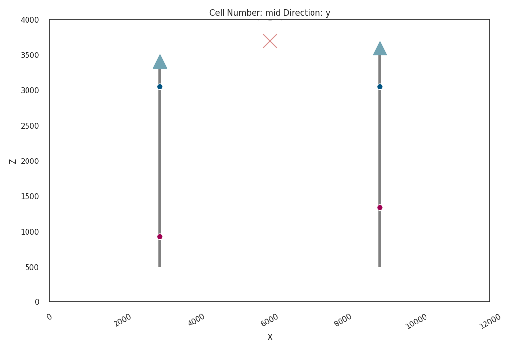
Define a function for plotting geological settings with wells

def plot_geo_setting_well(geo_model, alpha=1., show_lith=True):
    """
    This function plots the geological settings along with the well locations.
    It uses gempy_viewer to create 2D plots of the model.
    """
    # Define well and device locations
    device_loc = np.array([[6e3, 0, 3700]])
    well_1 = 3.41e3
    well_2 = 3.6e3

    # Create a 2D plot
    p2d = gpv.plot_2d(
        geo_model,
        show_topography=False,
        legend=False,
        show=False,
        show_lith=show_lith,
        kwargs_boundaries={'alpha': alpha}
    )

    # Add well and device markers to the plot
    p2d.axes[0].scatter([3e3], [well_1], marker='^', s=400, c='#71a4b3', zorder=10)
    p2d.axes[0].scatter([9e3], [well_2], marker='^', s=400, c='#71a4b3', zorder=10)
    p2d.axes[0].scatter(device_loc[:, 0], device_loc[:, 2], marker='x', s=400, c='#DA8886', zorder=10)

    # Add vertical lines to represent wells
    p2d.axes[0].vlines(3e3, .5e3, well_1, linewidth=4, color='gray')
    p2d.axes[0].vlines(9e3, .5e3, well_2, linewidth=4, color='gray')

    # Show the plot
    p2d.fig.show()
    return p2d

Creating the Geological Model

Here we create a geological model using GemPy. The model defines the spatial extent, resolution, and geological information derived from orientations and surface points data.

geo_model = gp.create_geomodel(
    project_name='Wells',
    extent=[0, 12000, -500, 500, 0, 4000],
    resolution=[100, 2, 100],
    # refinement=1,
    importer_helper=gp.data.ImporterHelper(
        path_to_orientations=data_path + "/data/2-layers/2-layers_orientations.csv",
        path_to_surface_points=data_path + "/data/2-layers/2-layers_surface_points.csv"
    )
)

Configuring the Model

We configure the interpolation options for the geological model. These options determine how the model interpolates between data points.

geo_model.interpolation_options.uni_degree = 1
geo_model.interpolation_options.mesh_extraction = False
geo_model.interpolation_options.sigmoid_slope = 1000  # ! Temporary fix to set the hard sigmoid

Setting up a Custom Grid

A custom grid is set for the model, defining specific points in space where geological formations will be evaluated.

x_loc = 6000
y_loc = 0
z_loc = np.linspace(0, 4000, 100)
xyz_coord = np.array([[x_loc, y_loc, z] for z in z_loc])
gp.set_custom_grid(geo_model.grid, xyz_coord=xyz_coord)

Active grids: GridTypes.NONE|CUSTOM|DENSE

<gempy.core.data.grid_modules.grid_types.CustomGrid object at 0x7f27af42b850>

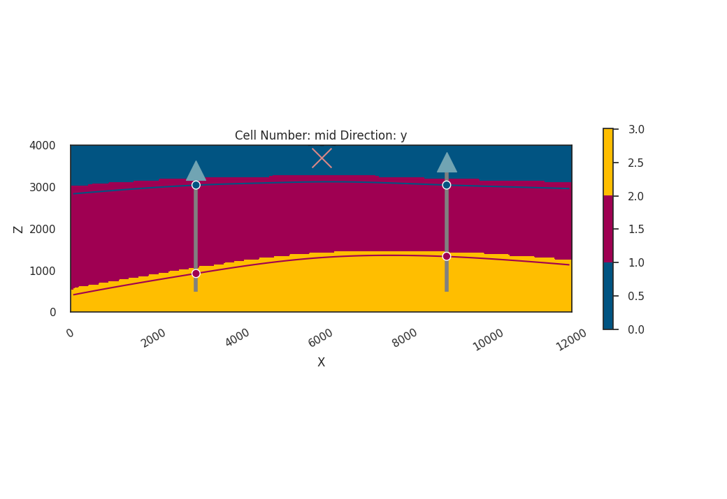
Plotting the Initial Geological Setting

Before running any probabilistic analysis, we first visualize the initial geological setting. This step ensures that our model is correctly set up with the initial data.

# Plot initial geological settings
plot_geo_setting_well(geo_model=geo_model)

<gempy_viewer.modules.plot_2d.visualization_2d.Plot2D object at 0x7f280b0e6f80>

Interpolating the Initial Guess

The model interpolates an initial guess for the geological formations. This step is crucial to provide a starting point for further probabilistic analysis.

gp.compute_model(
    gempy_model=geo_model,
    engine_config=gp.data.GemPyEngineConfig(backend=gp.data.AvailableBackends.numpy)
)
plot_geo_setting_well(geo_model=geo_model)

Setting Backend To: AvailableBackends.numpy

<gempy_viewer.modules.plot_2d.visualization_2d.Plot2D object at 0x7f27ad1b15a0>

Probabilistic Geomodeling with Pyro

In this section, we introduce a probabilistic approach to geological modeling. By using Pyro, a probabilistic programming language, we define a model that integrates geological data with uncertainty quantification.

sp_coords_copy = geo_model.interpolation_input_copy.surface_points.sp_coords.copy()
# Change the backend to PyTorch for probabilistic modeling
BackendTensor.change_backend_gempy(engine_backend=gp.data.AvailableBackends.PYTORCH)

Setting Backend To: AvailableBackends.PYTORCH

Defining the Probabilistic Model

The Pyro model represents the probabilistic aspects of the geological model. It defines a prior distribution for the top layer’s location and computes the thickness of the geological layer as an observed variable.

def model(y_obs_list):
    """
    This Pyro model represents the probabilistic aspects of the geological model.
    It defines a prior distribution for the top layer's location and
    computes the thickness of the geological layer as an observed variable.
    """
    # Define prior for the top layer's location
    prior_mean = sp_coords_copy[0, 2]
    mu_top = pyro.sample(
        name=r'$\mu_{top}$',
        fn=dist.Normal(prior_mean, torch.tensor(0.02, dtype=torch.float64))
    )

    # Update the model with the new top layer's location
    interpolation_input = geo_model.interpolation_input_copy
    interpolation_input.surface_points.sp_coords = torch.index_put(
        interpolation_input.surface_points.sp_coords,
        (torch.tensor([0]), torch.tensor([2])),
        mu_top
    )

    # Compute the geological model
    geo_model.solutions = gempy_engine.compute_model(
        interpolation_input=interpolation_input,
        options=geo_model.interpolation_options,
        data_descriptor=geo_model.input_data_descriptor,
        geophysics_input=geo_model.geophysics_input,
    )

    # Compute and observe the thickness of the geological layer
    simulated_well = geo_model.solutions.octrees_output[0].last_output_center.custom_grid_values
    thickness = simulated_well.sum()
    pyro.deterministic(r'$\mu_{thickness}$', thickness.detach())
    y_thickness = pyro.sample(r'$y_{thickness}$', dist.Normal(thickness, 50), obs=y_obs_list)

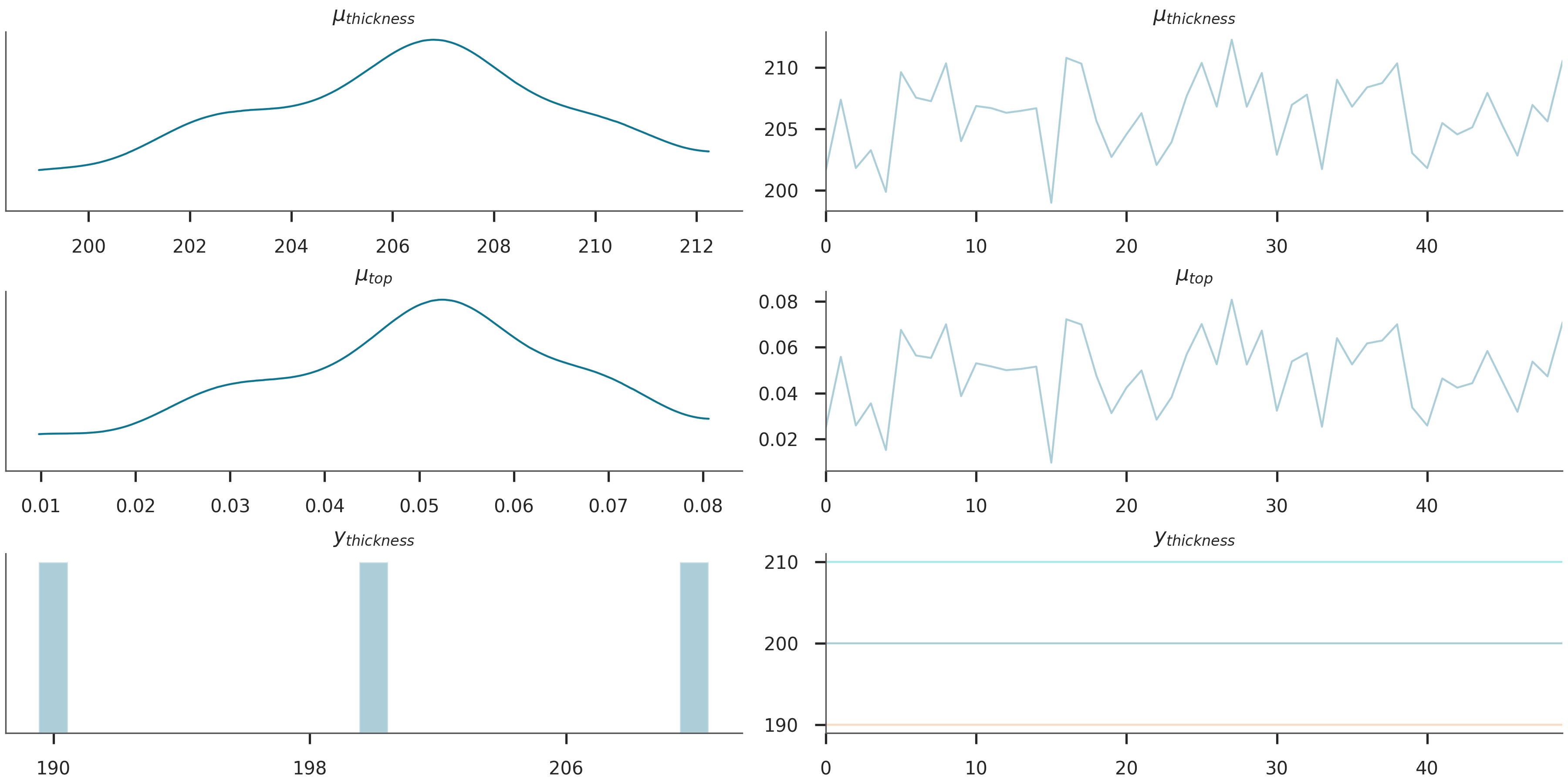
Running Prior Sampling and Visualization

Prior sampling is an essential step in probabilistic modeling. It helps in understanding the distribution of our prior assumptions before observing any data.

Prepare observation data

y_obs_list = torch.tensor([200, 210, 190])

Run prior sampling and visualization

prior = Predictive(model, num_samples=50)(y_obs_list)
data = az.from_pyro(prior=prior)
az.plot_trace(data.prior)
plt.show()

Sampling from the Posterior using MCMC

We use Markov Chain Monte Carlo (MCMC) with the NUTS (No-U-Turn Sampler) algorithm to sample from the posterior distribution. This gives us an understanding of the distribution of our model parameters after considering the observed data.

Run MCMC using NUTS to sample from the posterior

# Magic sauce
from gempy_engine.core.backend_tensor import BackendTensor

# import gempy_engine.config
# config.DEFAULT_PYKEOPS = False
BackendTensor._change_backend(
    engine_backend=gp.data.AvailableBackends.PYTORCH,
    dtype="float64",
    pykeops_enabled=False
)

pyro.primitives.enable_validation(is_validate=True)
nuts_kernel = NUTS(model, step_size=0.0085, adapt_step_size=True, target_accept_prob=0.9, max_tree_depth=10, init_strategy=init_to_mean)
mcmc = MCMC(nuts_kernel, num_samples=200, warmup_steps=50)
mcmc.run(y_obs_list)

Setting Backend To: AvailableBackends.PYTORCH

Warmup:   0%|          | 0/250 [00:00, ?it/s]
Warmup:   0%|          | 1/250 [00:00,  1.31it/s, step size=1.32e-01, acc. prob=0.000]
Warmup:   2%|▏         | 4/250 [00:01,  3.83it/s, step size=6.85e-03, acc. prob=0.498]
Warmup:   2%|▏         | 5/250 [00:01,  3.50it/s, step size=6.86e-03, acc. prob=0.592]
Warmup:   2%|▏         | 6/250 [00:01,  4.21it/s, step size=8.19e-03, acc. prob=0.659]
Warmup:   3%|▎         | 7/250 [00:01,  4.15it/s, step size=9.21e-03, acc. prob=0.703]
Warmup:   3%|▎         | 8/250 [00:02,  4.95it/s, step size=9.81e-03, acc. prob=0.731]
Warmup:   4%|▎         | 9/250 [00:02,  5.77it/s, step size=1.27e-02, acc. prob=0.760]
Warmup:   4%|▍         | 10/250 [00:02,  5.12it/s, step size=1.70e-02, acc. prob=0.783]
Warmup:   4%|▍         | 11/250 [00:02,  4.73it/s, step size=2.34e-02, acc. prob=0.803]
Warmup:   5%|▍         | 12/250 [00:02,  5.56it/s, step size=1.94e-02, acc. prob=0.806]
Warmup:   5%|▌         | 13/250 [00:02,  6.17it/s, step size=1.92e-02, acc. prob=0.813]
Warmup:   6%|▋         | 16/250 [00:02, 10.85it/s, step size=1.80e-02, acc. prob=0.826]
Warmup:   8%|▊         | 19/250 [00:03, 14.95it/s, step size=2.88e-02, acc. prob=0.845]
Warmup:   9%|▉         | 22/250 [00:03, 18.46it/s, step size=3.42e-03, acc. prob=0.818]
Warmup:  10%|█         | 25/250 [00:04,  5.78it/s, step size=8.64e-03, acc. prob=0.839]
Warmup:  11%|█         | 27/250 [00:04,  6.82it/s, step size=1.45e-02, acc. prob=0.849]
Warmup:  12%|█▏        | 29/250 [00:04,  5.82it/s, step size=1.89e-02, acc. prob=0.855]
Warmup:  12%|█▏        | 31/250 [00:05,  6.61it/s, step size=3.36e-02, acc. prob=0.864]
Warmup:  13%|█▎        | 33/250 [00:05,  7.81it/s, step size=9.68e-03, acc. prob=0.852]
Warmup:  14%|█▍        | 35/250 [00:05,  8.99it/s, step size=1.74e-02, acc. prob=0.860]
Warmup:  15%|█▍        | 37/250 [00:05,  7.80it/s, step size=1.31e-02, acc. prob=0.859]
Warmup:  16%|█▌        | 39/250 [00:06,  7.76it/s, step size=2.29e-02, acc. prob=0.866]
Warmup:  16%|█▌        | 40/250 [00:06,  8.03it/s, step size=3.03e-02, acc. prob=0.869]
Warmup:  17%|█▋        | 42/250 [00:06,  7.73it/s, step size=9.41e-03, acc. prob=0.859]
Warmup:  17%|█▋        | 43/250 [00:06,  6.77it/s, step size=1.22e-02, acc. prob=0.862]
Warmup:  18%|█▊        | 44/250 [00:07,  3.86it/s, step size=2.01e+00, acc. prob=0.865]
Warmup:  19%|█▉        | 47/250 [00:07,  5.39it/s, step size=3.15e-01, acc. prob=0.834]
Warmup:  19%|█▉        | 48/250 [00:07,  4.98it/s, step size=3.07e-01, acc. prob=0.838]
Warmup:  20%|█▉        | 49/250 [00:07,  5.46it/s, step size=4.44e-01, acc. prob=0.841]
Warmup:  20%|██        | 50/250 [00:08,  4.97it/s, step size=4.44e-01, acc. prob=0.843]
Warmup:  20%|██        | 51/250 [00:08,  4.62it/s, step size=4.44e-01, acc. prob=0.967]
Sample:  21%|██        | 52/250 [00:08,  4.19it/s, step size=4.44e-01, acc. prob=0.983]
Sample:  21%|██        | 53/250 [00:09,  3.84it/s, step size=4.44e-01, acc. prob=0.971]
Sample:  22%|██▏       | 54/250 [00:09,  4.49it/s, step size=4.44e-01, acc. prob=0.978]
Sample:  22%|██▏       | 55/250 [00:09,  5.22it/s, step size=4.44e-01, acc. prob=0.981]
Sample:  22%|██▏       | 56/250 [00:09,  4.80it/s, step size=4.44e-01, acc. prob=0.984]
Sample:  23%|██▎       | 57/250 [00:09,  4.77it/s, step size=4.44e-01, acc. prob=0.983]
Sample:  23%|██▎       | 58/250 [00:10,  4.28it/s, step size=4.44e-01, acc. prob=0.986]
Sample:  24%|██▎       | 59/250 [00:10,  4.91it/s, step size=4.44e-01, acc. prob=0.987]
Sample:  24%|██▍       | 60/250 [00:10,  5.41it/s, step size=4.44e-01, acc. prob=0.988]
Sample:  24%|██▍       | 61/250 [00:10,  4.37it/s, step size=4.44e-01, acc. prob=0.979]
Sample:  26%|██▌       | 64/250 [00:10,  7.32it/s, step size=4.44e-01, acc. prob=0.984]
Sample:  26%|██▌       | 65/250 [00:11,  7.48it/s, step size=4.44e-01, acc. prob=0.984]
Sample:  26%|██▋       | 66/250 [00:11,  6.24it/s, step size=4.44e-01, acc. prob=0.985]
Sample:  27%|██▋       | 67/250 [00:11,  6.77it/s, step size=4.44e-01, acc. prob=0.984]
Sample:  27%|██▋       | 68/250 [00:11,  5.77it/s, step size=4.44e-01, acc. prob=0.984]
Sample:  28%|██▊       | 69/250 [00:11,  6.46it/s, step size=4.44e-01, acc. prob=0.984]
Sample:  28%|██▊       | 70/250 [00:12,  5.49it/s, step size=4.44e-01, acc. prob=0.985]
Sample:  28%|██▊       | 71/250 [00:12,  6.22it/s, step size=4.44e-01, acc. prob=0.984]
Sample:  29%|██▉       | 73/250 [00:12,  8.28it/s, step size=4.44e-01, acc. prob=0.985]
Sample:  30%|███       | 75/250 [00:12,  9.76it/s, step size=4.44e-01, acc. prob=0.986]
Sample:  31%|███       | 77/250 [00:12,  7.69it/s, step size=4.44e-01, acc. prob=0.986]
Sample:  31%|███       | 78/250 [00:12,  7.99it/s, step size=4.44e-01, acc. prob=0.984]
Sample:  32%|███▏      | 79/250 [00:13,  6.42it/s, step size=4.44e-01, acc. prob=0.982]
Sample:  32%|███▏      | 80/250 [00:13,  5.61it/s, step size=4.44e-01, acc. prob=0.983]
Sample:  32%|███▏      | 81/250 [00:13,  6.31it/s, step size=4.44e-01, acc. prob=0.983]
Sample:  33%|███▎      | 82/250 [00:13,  5.43it/s, step size=4.44e-01, acc. prob=0.984]
Sample:  33%|███▎      | 83/250 [00:13,  6.16it/s, step size=4.44e-01, acc. prob=0.984]
Sample:  34%|███▎      | 84/250 [00:14,  5.45it/s, step size=4.44e-01, acc. prob=0.984]
Sample:  34%|███▍      | 85/250 [00:14,  5.46it/s, step size=4.44e-01, acc. prob=0.984]
Sample:  34%|███▍      | 86/250 [00:14,  4.84it/s, step size=4.44e-01, acc. prob=0.985]
Sample:  35%|███▍      | 87/250 [00:14,  5.61it/s, step size=4.44e-01, acc. prob=0.985]
Sample:  36%|███▌      | 89/250 [00:14,  6.09it/s, step size=4.44e-01, acc. prob=0.986]
Sample:  36%|███▌      | 90/250 [00:15,  5.90it/s, step size=4.44e-01, acc. prob=0.985]
Sample:  36%|███▋      | 91/250 [00:15,  5.23it/s, step size=4.44e-01, acc. prob=0.985]
Sample:  37%|███▋      | 92/250 [00:15,  5.92it/s, step size=4.44e-01, acc. prob=0.986]
Sample:  37%|███▋      | 93/250 [00:15,  6.57it/s, step size=4.44e-01, acc. prob=0.986]
Sample:  38%|███▊      | 94/250 [00:15,  5.53it/s, step size=4.44e-01, acc. prob=0.986]
Sample:  38%|███▊      | 95/250 [00:16,  5.43it/s, step size=4.44e-01, acc. prob=0.986]
Sample:  39%|███▉      | 97/250 [00:16,  5.89it/s, step size=4.44e-01, acc. prob=0.986]
Sample:  39%|███▉      | 98/250 [00:16,  5.27it/s, step size=4.44e-01, acc. prob=0.986]
Sample:  40%|███▉      | 99/250 [00:16,  4.89it/s, step size=4.44e-01, acc. prob=0.987]
Sample:  40%|████      | 100/250 [00:17,  4.54it/s, step size=4.44e-01, acc. prob=0.987]
Sample:  40%|████      | 101/250 [00:17,  4.77it/s, step size=4.44e-01, acc. prob=0.987]
Sample:  41%|████      | 102/250 [00:17,  4.98it/s, step size=4.44e-01, acc. prob=0.987]
Sample:  41%|████      | 103/250 [00:17,  5.72it/s, step size=4.44e-01, acc. prob=0.987]
Sample:  42%|████▏     | 104/250 [00:17,  5.69it/s, step size=4.44e-01, acc. prob=0.987]
Sample:  42%|████▏     | 105/250 [00:18,  4.98it/s, step size=4.44e-01, acc. prob=0.987]
Sample:  43%|████▎     | 108/250 [00:18,  9.15it/s, step size=4.44e-01, acc. prob=0.987]
Sample:  44%|████▍     | 111/250 [00:18, 11.43it/s, step size=4.44e-01, acc. prob=0.987]
Sample:  45%|████▌     | 113/250 [00:18,  8.63it/s, step size=4.44e-01, acc. prob=0.986]
Sample:  46%|████▌     | 115/250 [00:19,  5.90it/s, step size=4.44e-01, acc. prob=0.987]
Sample:  46%|████▋     | 116/250 [00:19,  6.30it/s, step size=4.44e-01, acc. prob=0.987]
Sample:  47%|████▋     | 117/250 [00:19,  5.55it/s, step size=4.44e-01, acc. prob=0.987]
Sample:  48%|████▊     | 120/250 [00:19,  7.96it/s, step size=4.44e-01, acc. prob=0.987]
Sample:  48%|████▊     | 121/250 [00:20,  6.74it/s, step size=4.44e-01, acc. prob=0.987]
Sample:  49%|████▉     | 122/250 [00:20,  5.83it/s, step size=4.44e-01, acc. prob=0.987]
Sample:  49%|████▉     | 123/250 [00:20,  5.79it/s, step size=4.44e-01, acc. prob=0.987]
Sample:  50%|████▉     | 124/250 [00:20,  5.64it/s, step size=4.44e-01, acc. prob=0.987]
Sample:  50%|█████     | 125/250 [00:20,  5.02it/s, step size=4.44e-01, acc. prob=0.987]
Sample:  50%|█████     | 126/250 [00:21,  3.41it/s, step size=4.44e-01, acc. prob=0.987]
Sample:  51%|█████     | 128/250 [00:21,  4.35it/s, step size=4.44e-01, acc. prob=0.987]
Sample:  52%|█████▏    | 129/250 [00:21,  4.95it/s, step size=4.44e-01, acc. prob=0.987]
Sample:  52%|█████▏    | 130/250 [00:22,  4.62it/s, step size=4.44e-01, acc. prob=0.987]
Sample:  52%|█████▏    | 131/250 [00:22,  4.45it/s, step size=4.44e-01, acc. prob=0.987]
Sample:  53%|█████▎    | 132/250 [00:22,  4.36it/s, step size=4.44e-01, acc. prob=0.987]
Sample:  53%|█████▎    | 133/250 [00:22,  4.32it/s, step size=4.44e-01, acc. prob=0.987]
Sample:  54%|█████▎    | 134/250 [00:23,  5.13it/s, step size=4.44e-01, acc. prob=0.987]
Sample:  54%|█████▍    | 135/250 [00:23,  5.90it/s, step size=4.44e-01, acc. prob=0.987]
Sample:  55%|█████▍    | 137/250 [00:23,  6.32it/s, step size=4.44e-01, acc. prob=0.987]
Sample:  55%|█████▌    | 138/250 [00:23,  5.54it/s, step size=4.44e-01, acc. prob=0.987]
Sample:  56%|█████▌    | 139/250 [00:23,  6.14it/s, step size=4.44e-01, acc. prob=0.987]
Sample:  56%|█████▌    | 140/250 [00:23,  6.71it/s, step size=4.44e-01, acc. prob=0.987]
Sample:  56%|█████▋    | 141/250 [00:24,  5.61it/s, step size=4.44e-01, acc. prob=0.987]
Sample:  57%|█████▋    | 142/250 [00:24,  4.99it/s, step size=4.44e-01, acc. prob=0.986]
Sample:  57%|█████▋    | 143/250 [00:24,  4.63it/s, step size=4.44e-01, acc. prob=0.987]
Sample:  58%|█████▊    | 144/250 [00:24,  5.42it/s, step size=4.44e-01, acc. prob=0.987]
Sample:  58%|█████▊    | 145/250 [00:24,  5.42it/s, step size=4.44e-01, acc. prob=0.987]
Sample:  58%|█████▊    | 146/250 [00:25,  4.82it/s, step size=4.44e-01, acc. prob=0.987]
Sample:  59%|█████▉    | 147/250 [00:25,  5.57it/s, step size=4.44e-01, acc. prob=0.987]
Sample:  59%|█████▉    | 148/250 [00:25,  4.94it/s, step size=4.44e-01, acc. prob=0.987]
Sample:  60%|█████▉    | 149/250 [00:25,  5.72it/s, step size=4.44e-01, acc. prob=0.987]
Sample:  60%|██████    | 150/250 [00:25,  6.41it/s, step size=4.44e-01, acc. prob=0.986]
Sample:  61%|██████    | 152/250 [00:26,  7.40it/s, step size=4.44e-01, acc. prob=0.986]
Sample:  61%|██████    | 153/250 [00:26,  6.02it/s, step size=4.44e-01, acc. prob=0.986]
Sample:  62%|██████▏   | 154/250 [00:26,  5.29it/s, step size=4.44e-01, acc. prob=0.986]
Sample:  62%|██████▏   | 156/250 [00:26,  5.78it/s, step size=4.44e-01, acc. prob=0.987]
Sample:  63%|██████▎   | 157/250 [00:27,  5.69it/s, step size=4.44e-01, acc. prob=0.986]
Sample:  63%|██████▎   | 158/250 [00:27,  5.13it/s, step size=4.44e-01, acc. prob=0.986]
Sample:  64%|██████▎   | 159/250 [00:27,  4.74it/s, step size=4.44e-01, acc. prob=0.986]
Sample:  64%|██████▍   | 160/250 [00:27,  4.90it/s, step size=4.44e-01, acc. prob=0.986]
Sample:  64%|██████▍   | 161/250 [00:27,  4.53it/s, step size=4.44e-01, acc. prob=0.986]
Sample:  65%|██████▍   | 162/250 [00:28,  5.29it/s, step size=4.44e-01, acc. prob=0.986]
Sample:  65%|██████▌   | 163/250 [00:28,  6.01it/s, step size=4.44e-01, acc. prob=0.986]
Sample:  66%|██████▌   | 164/250 [00:28,  3.58it/s, step size=4.44e-01, acc. prob=0.986]
Sample:  66%|██████▌   | 165/250 [00:28,  3.99it/s, step size=4.44e-01, acc. prob=0.986]
Sample:  67%|██████▋   | 167/250 [00:29,  4.92it/s, step size=4.44e-01, acc. prob=0.986]
Sample:  67%|██████▋   | 168/250 [00:29,  4.60it/s, step size=4.44e-01, acc. prob=0.986]
Sample:  68%|██████▊   | 169/250 [00:29,  4.43it/s, step size=4.44e-01, acc. prob=0.986]
Sample:  68%|██████▊   | 170/250 [00:29,  4.31it/s, step size=4.44e-01, acc. prob=0.986]
Sample:  68%|██████▊   | 171/250 [00:30,  4.21it/s, step size=4.44e-01, acc. prob=0.986]
Sample:  69%|██████▉   | 172/250 [00:30,  4.12it/s, step size=4.44e-01, acc. prob=0.986]
Sample:  69%|██████▉   | 173/250 [00:30,  4.91it/s, step size=4.44e-01, acc. prob=0.986]
Sample:  70%|██████▉   | 174/250 [00:30,  5.68it/s, step size=4.44e-01, acc. prob=0.986]
Sample:  70%|███████   | 175/250 [00:30,  6.36it/s, step size=4.44e-01, acc. prob=0.986]
Sample:  70%|███████   | 176/250 [00:30,  6.97it/s, step size=4.44e-01, acc. prob=0.986]
Sample:  71%|███████   | 177/250 [00:31,  6.45it/s, step size=4.44e-01, acc. prob=0.986]
Sample:  71%|███████   | 178/250 [00:31,  5.41it/s, step size=4.44e-01, acc. prob=0.986]
Sample:  72%|███████▏  | 179/250 [00:31,  5.44it/s, step size=4.44e-01, acc. prob=0.986]
Sample:  73%|███████▎  | 182/250 [00:31,  6.98it/s, step size=4.44e-01, acc. prob=0.986]
Sample:  73%|███████▎  | 183/250 [00:32,  6.57it/s, step size=4.44e-01, acc. prob=0.986]
Sample:  74%|███████▎  | 184/250 [00:32,  5.72it/s, step size=4.44e-01, acc. prob=0.986]
Sample:  74%|███████▍  | 185/250 [00:32,  5.15it/s, step size=4.44e-01, acc. prob=0.986]
Sample:  74%|███████▍  | 186/250 [00:32,  5.87it/s, step size=4.44e-01, acc. prob=0.987]
Sample:  75%|███████▍  | 187/250 [00:32,  5.25it/s, step size=4.44e-01, acc. prob=0.986]
Sample:  75%|███████▌  | 188/250 [00:33,  5.92it/s, step size=4.44e-01, acc. prob=0.986]
Sample:  76%|███████▌  | 189/250 [00:33,  6.40it/s, step size=4.44e-01, acc. prob=0.986]
Sample:  76%|███████▌  | 190/250 [00:33,  5.43it/s, step size=4.44e-01, acc. prob=0.987]
Sample:  76%|███████▋  | 191/250 [00:33,  6.20it/s, step size=4.44e-01, acc. prob=0.987]
Sample:  77%|███████▋  | 192/250 [00:33,  5.36it/s, step size=4.44e-01, acc. prob=0.987]
Sample:  78%|███████▊  | 194/250 [00:33,  7.44it/s, step size=4.44e-01, acc. prob=0.987]
Sample:  78%|███████▊  | 195/250 [00:34,  6.04it/s, step size=4.44e-01, acc. prob=0.987]
Sample:  78%|███████▊  | 196/250 [00:34,  5.31it/s, step size=4.44e-01, acc. prob=0.987]
Sample:  79%|███████▉  | 197/250 [00:34,  5.38it/s, step size=4.44e-01, acc. prob=0.987]
Sample:  80%|███████▉  | 199/250 [00:34,  7.31it/s, step size=4.44e-01, acc. prob=0.987]
Sample:  80%|████████  | 200/250 [00:35,  6.07it/s, step size=4.44e-01, acc. prob=0.987]
Sample:  80%|████████  | 201/250 [00:35,  6.67it/s, step size=4.44e-01, acc. prob=0.987]
Sample:  81%|████████  | 202/250 [00:35,  7.20it/s, step size=4.44e-01, acc. prob=0.987]
Sample:  82%|████████▏ | 204/250 [00:35,  9.08it/s, step size=4.44e-01, acc. prob=0.986]
Sample:  82%|████████▏ | 205/250 [00:35,  6.95it/s, step size=4.44e-01, acc. prob=0.986]
Sample:  82%|████████▏ | 206/250 [00:35,  7.41it/s, step size=4.44e-01, acc. prob=0.987]
Sample:  83%|████████▎ | 207/250 [00:35,  6.74it/s, step size=4.44e-01, acc. prob=0.987]
Sample:  83%|████████▎ | 208/250 [00:36,  5.62it/s, step size=4.44e-01, acc. prob=0.986]
Sample:  84%|████████▎ | 209/250 [00:36,  4.98it/s, step size=4.44e-01, acc. prob=0.986]
Sample:  84%|████████▍ | 210/250 [00:36,  3.34it/s, step size=4.44e-01, acc. prob=0.986]
Sample:  84%|████████▍ | 211/250 [00:37,  4.11it/s, step size=4.44e-01, acc. prob=0.986]
Sample:  85%|████████▍ | 212/250 [00:37,  4.88it/s, step size=4.44e-01, acc. prob=0.986]
Sample:  85%|████████▌ | 213/250 [00:37,  4.49it/s, step size=4.44e-01, acc. prob=0.986]
Sample:  86%|████████▋ | 216/250 [00:37,  7.46it/s, step size=4.44e-01, acc. prob=0.986]
Sample:  87%|████████▋ | 217/250 [00:37,  7.72it/s, step size=4.44e-01, acc. prob=0.987]
Sample:  87%|████████▋ | 218/250 [00:37,  8.04it/s, step size=4.44e-01, acc. prob=0.987]
Sample:  88%|████████▊ | 219/250 [00:37,  8.30it/s, step size=4.44e-01, acc. prob=0.987]
Sample:  88%|████████▊ | 220/250 [00:38,  7.43it/s, step size=4.44e-01, acc. prob=0.987]
Sample:  88%|████████▊ | 221/250 [00:38,  7.82it/s, step size=4.44e-01, acc. prob=0.987]
Sample:  89%|████████▉ | 222/250 [00:38,  8.12it/s, step size=4.44e-01, acc. prob=0.987]
Sample:  89%|████████▉ | 223/250 [00:38,  7.12it/s, step size=4.44e-01, acc. prob=0.986]
Sample:  90%|█████████ | 226/250 [00:39,  5.49it/s, step size=4.44e-01, acc. prob=0.987]
Sample:  91%|█████████ | 227/250 [00:39,  5.04it/s, step size=4.44e-01, acc. prob=0.987]
Sample:  91%|█████████ | 228/250 [00:39,  4.73it/s, step size=4.44e-01, acc. prob=0.987]
Sample:  92%|█████████▏| 229/250 [00:39,  5.37it/s, step size=4.44e-01, acc. prob=0.987]
Sample:  92%|█████████▏| 230/250 [00:40,  5.32it/s, step size=4.44e-01, acc. prob=0.987]
Sample:  92%|█████████▏| 231/250 [00:40,  4.86it/s, step size=4.44e-01, acc. prob=0.987]
Sample:  93%|█████████▎| 232/250 [00:40,  4.51it/s, step size=4.44e-01, acc. prob=0.987]
Sample:  93%|█████████▎| 233/250 [00:40,  4.32it/s, step size=4.44e-01, acc. prob=0.987]
Sample:  94%|█████████▎| 234/250 [00:41,  4.27it/s, step size=4.44e-01, acc. prob=0.987]
Sample:  94%|█████████▍| 235/250 [00:41,  4.65it/s, step size=4.44e-01, acc. prob=0.987]
Sample:  94%|█████████▍| 236/250 [00:41,  4.51it/s, step size=4.44e-01, acc. prob=0.987]
Sample:  95%|█████████▍| 237/250 [00:41,  5.38it/s, step size=4.44e-01, acc. prob=0.987]
Sample:  95%|█████████▌| 238/250 [00:41,  6.16it/s, step size=4.44e-01, acc. prob=0.987]
Sample:  96%|█████████▌| 240/250 [00:41,  6.41it/s, step size=4.44e-01, acc. prob=0.987]
Sample:  96%|█████████▋| 241/250 [00:42,  5.90it/s, step size=4.44e-01, acc. prob=0.987]
Sample:  97%|█████████▋| 242/250 [00:42,  5.57it/s, step size=4.44e-01, acc. prob=0.986]
Sample:  97%|█████████▋| 243/250 [00:42,  4.91it/s, step size=4.44e-01, acc. prob=0.986]
Sample:  98%|█████████▊| 244/250 [00:42,  4.49it/s, step size=4.44e-01, acc. prob=0.986]
Sample:  98%|█████████▊| 245/250 [00:43,  3.86it/s, step size=4.44e-01, acc. prob=0.986]
Sample:  98%|█████████▊| 246/250 [00:43,  3.41it/s, step size=4.44e-01, acc. prob=0.986]
Sample:  99%|█████████▉| 248/250 [00:43,  4.25it/s, step size=4.44e-01, acc. prob=0.986]
Sample: 100%|█████████▉| 249/250 [00:44,  4.19it/s, step size=4.44e-01, acc. prob=0.986]
Sample: 100%|██████████| 250/250 [00:44,  4.12it/s, step size=4.44e-01, acc. prob=0.986]
Sample: 100%|██████████| 250/250 [00:44,  5.62it/s, step size=4.44e-01, acc. prob=0.986]

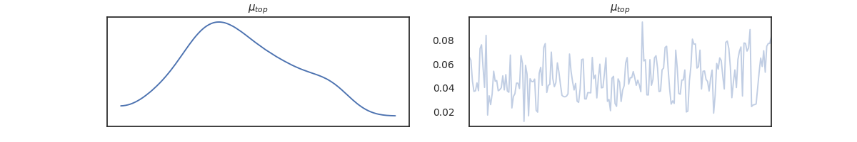
Posterior Predictive Checks

After obtaining the posterior samples, we perform posterior predictive checks. This step is crucial to evaluate the performance and validity of our probabilistic model.

Sample from posterior predictive and visualize

posterior_samples = mcmc.get_samples()
posterior_predictive = Predictive(model, posterior_samples)(y_obs_list)
data = az.from_pyro(posterior=mcmc, prior=prior, posterior_predictive=posterior_predictive)
az.plot_trace(data)
plt.show()

/home/leguark/.virtualenvs/gempy_dependencies/lib/python3.10/site-packages/arviz/data/io_pyro.py:158: UserWarning: Could not get vectorized trace, log_likelihood group will be omitted. Check your model vectorization or set log_likelihood=False
  warnings.warn(

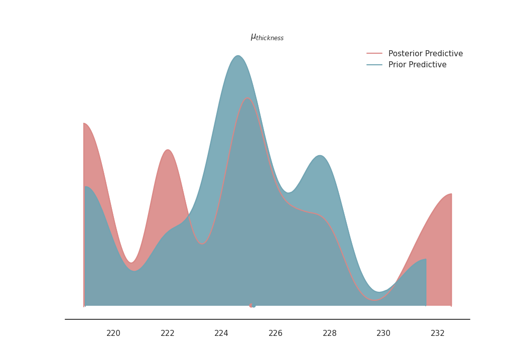
Density Plot of Posterior Predictive

A density plot provides a visual representation of the distribution of the posterior predictive checks. It helps in comparing the prior and posterior distributions and in assessing the impact of our observed data on the model.

Plot density of posterior predictive and prior predictive

az.plot_density(
    data=[data.posterior_predictive, data.prior_predictive],
    shade=.9,
    var_names=[r'$\mu_{thickness}$'],
    data_labels=["Posterior Predictive", "Prior Predictive"],
    colors=[default_red, default_blue],
)
plt.show()

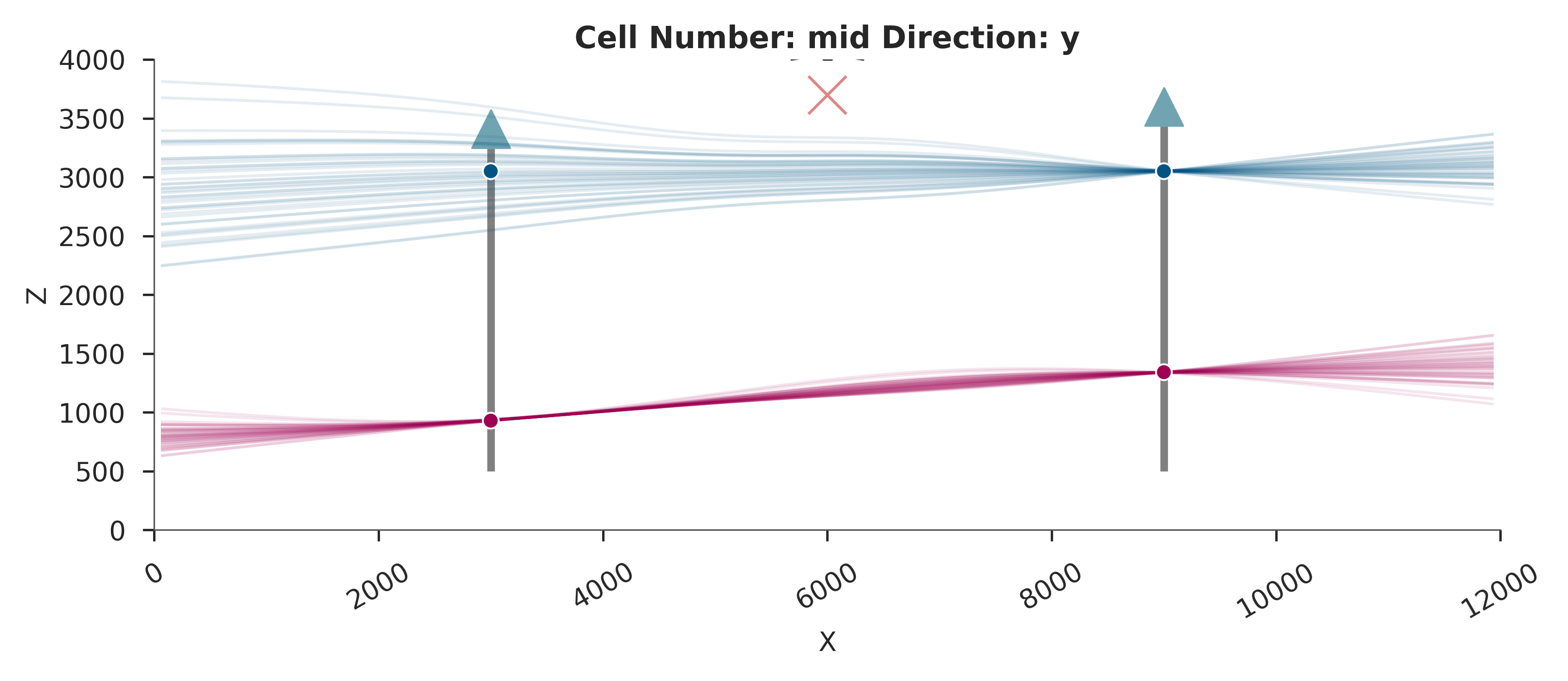
Plot spagetti

p2d = plot_geo_setting_well(geo_model, alpha=0.1, show_lith=False)
for i in range(0,199,5):
    gp.modify_surface_points(
        geo_model=geo_model,
        slice=0,
        Z= geo_model.input_transform.apply_inverse(
            points=np.array([[0, 0, data.posterior[r'$\mu_{top}$'][0][i].item()]]))[0,2]
    )

    gp.compute_model(geo_model)

    plot_regular_grid_contacts(
        gempy_model=geo_model,
        ax=p2d.axes[0],
        slicer_data=p2d.section_data_list[0].slicer_data,
        resolution=geo_model.grid.regular_grid.resolution,
        only_faults=False,
        kwargs={'alpha': 0.1}
    )

p2d.fig.show()

# sphinx_gallery_thumbnail_number = 2

Setting Backend To: AvailableBackends.numpy
Setting Backend To: AvailableBackends.numpy
Setting Backend To: AvailableBackends.numpy
Setting Backend To: AvailableBackends.numpy
Setting Backend To: AvailableBackends.numpy
Setting Backend To: AvailableBackends.numpy
Setting Backend To: AvailableBackends.numpy
Setting Backend To: AvailableBackends.numpy
Setting Backend To: AvailableBackends.numpy
Setting Backend To: AvailableBackends.numpy
Setting Backend To: AvailableBackends.numpy
Setting Backend To: AvailableBackends.numpy
Setting Backend To: AvailableBackends.numpy
Setting Backend To: AvailableBackends.numpy
Setting Backend To: AvailableBackends.numpy
Setting Backend To: AvailableBackends.numpy
Setting Backend To: AvailableBackends.numpy
Setting Backend To: AvailableBackends.numpy
Setting Backend To: AvailableBackends.numpy
Setting Backend To: AvailableBackends.numpy
Setting Backend To: AvailableBackends.numpy
Setting Backend To: AvailableBackends.numpy
Setting Backend To: AvailableBackends.numpy
Setting Backend To: AvailableBackends.numpy
Setting Backend To: AvailableBackends.numpy
Setting Backend To: AvailableBackends.numpy
Setting Backend To: AvailableBackends.numpy
Setting Backend To: AvailableBackends.numpy
Setting Backend To: AvailableBackends.numpy
Setting Backend To: AvailableBackends.numpy
Setting Backend To: AvailableBackends.numpy
Setting Backend To: AvailableBackends.numpy
Setting Backend To: AvailableBackends.numpy
Setting Backend To: AvailableBackends.numpy
Setting Backend To: AvailableBackends.numpy
Setting Backend To: AvailableBackends.numpy
Setting Backend To: AvailableBackends.numpy
Setting Backend To: AvailableBackends.numpy
Setting Backend To: AvailableBackends.numpy
Setting Backend To: AvailableBackends.numpy